
RESEARCH ARTICLE
Information Theoretic Quantification of Diagnostic Uncertainty
M Brandon Westover, Nathaniel A Eiseman, Sydney S Cash, Matt T Bianchi*
Article Information
Identifiers and Pagination:
Year: 2012Volume: 6
First Page: 36
Last Page: 50
Publisher Id: TOMINFOJ-6-36
DOI: 10.2174/1874431101206010036
Article History:
Received Date: 20/6/2012Revision Received Date: 19/8/2012
Acceptance Date: 21/8/2012
Electronic publication date: 14/12/2012
Collection year: 2012
open-access license: This is an open access article licensed under the terms of the Creative Commons Attribution Non-Commercial License (http://creativecommons.org/licenses/by-nc/3.0/) which permits unrestricted, non-commercial use, distribution and reproduction in any medium, provided the work is properly cited.
Abstract
Diagnostic test interpretation remains a challenge in clinical practice. Most physicians receive training in the use of Bayes’ rule, which specifies how the sensitivity and specificity of a test for a given disease combine with the pre-test probability to quantify the change in disease probability incurred by a new test result. However, multiple studies demonstrate physicians’ deficiencies in probabilistic reasoning, especially with unexpected test results. Information theory, a branch of probability theory dealing explicitly with the quantification of uncertainty, has been proposed as an alternative framework for diagnostic test interpretation, but is even less familiar to physicians. We have previously addressed one key challenge in the practical application of Bayes theorem: the handling of uncertainty in the critical first step of estimating the pre-test probability of disease. This essay aims to present the essential concepts of information theory to physicians in an accessible manner, and to extend previous work regarding uncertainty in pre-test probability estimation by placing this type of uncertainty within a principled information theoretic framework. We address several obstacles hindering physicians’ application of information theoretic concepts to diagnostic test interpretation. These include issues of terminology (mathematical meanings of certain information theoretic terms differ from clinical or common parlance) as well as the underlying mathematical assumptions. Finally, we illustrate how, in information theoretic terms, one can understand the effect on diagnostic uncertainty of considering ranges instead of simple point estimates of pre-test probability.
INTRODUCTION
The interpretation of diagnostic test results has been extensively discussed in the literature, and every physician receives training in the use of sensitivity, specificity, and predictive value calculations. Although it is recognized that neither diseases nor test results are dichotomous in reality, the essentials of interpretation are best understood (and taught) using the classic “2x2” box, which assumes yes/no possibilities. Bayes’ theorem is a formalization of test interpretation that utilizes the pre-test disease probability (pre-TP) and a given test result (positive or negative), to determine a new disease probability aptly called the post-test probability (post-TP) [1-3]. Although some suggest that physicians are natural Bayesians [4], many reports highlight deficiencies in formal or explicit probabilistic reasoning, including physician estimation of pre-TP, and the interpretation of test results in the context of pre-TP, particularly when results are unexpected (such as a positive result in a patient with low disease probability) [5-11]. One way to explicitly quantify the amount of uncertainty and how that uncertainty changes when we receive new information in diagnostic testing involves the use of information theory, introduced in the pioneering work of Shannon in 1948 in the context of communication theory [12]. Benish and others have elaborated strategies for understanding diagnostic tests in this context, but the information theoretic perspective has not enjoyed wide dissemination or implementation [13-18].
Four potential hurdles need to be addressed in order for information theory to gain traction among medical practitioners: 1) information theory is not routinely taught in medical curricula, 2) published resources applying information theory to diagnostics often involve mathematics unfamiliar to physicians, 3) the terminology used in information theory has vernacular implications that may differ from the precise mathematical concepts to which they refer, and 4) like Bayes’ theorem, there is little readily available guidance for handling ranges or confidence intervals in pre-TP, which may be described better as a qualitative impression than a precise estimate. Here, we address the latter three hurdles by providing intuitive explanations of information theoretic concepts, by relating the language of information theory to clinical parlance, and by developing an information theoretic approach to consider pre-TP as a range (instead of a point estimate) [19]. In this manner, we hope to render the application of information theory more relevant and practical for diagnostic interpretation.
TYPES OF UNCERTAINTY
“Uncertainty” has a variety of possible meanings that are context-specific, and various taxonomies of uncertainty have been described1. From the perspective of the physician’s background, sources of uncertainty may include knowledge base, training level, spectrum of experience, and so forth. In addition, the information conveyed by patients in the clinical history may contain uncertainty or ambiguity for any number of reasons.
From the perspective of diagnostic test interpretation, uncertainty can be understood in a more explicit manner. For example, if a physician estimates that a patient’s probability of disease is 20%, the diagnosis is, by definition, uncertain, because its probability is not zero or 100%. Mathematically, this uncertainty is modeled by casting the disease state as a random variable, D , which is assumed for simplicity to have one of two possible true values: D = 1 (“disease is present”) or D = 0 (“disease is absent”). Before testing, each of these two possibilities has an associated probability. Because we are interested clinically in the chance of disease, we speak particularly of probability of disease being present, known as the pre-TP, which is based on various clinical characteristics. Though it may appear at first cumbersome, it will be useful to introduce some additional formalism, to consider the pre-TP as a function. We thus specify a probability distribution function, g(d) , for each possible value d of D : for the probability that the disease is present ( D = 1) , we write g(1) = p , where p = the pre-TP, and for the probability that the disease is absent ( D = 0) , we write g(0) = 1- p . The advantages of this formalism will become apparent below when we introduce information theoretic concepts.
In addition, we can consider another level of uncertainty regarding the pre-TP: the pre-TP estimate itself is usually not precisely known, and thus the physician’s estimate may be captured better by a range of values, say, 20% ±5%. Thus, it may be appropriate to treat the pre-TP itself as a random variable, which we denote with a capital letter P . We may also specify the probability associated with each possible value of P within the permitted range, expressed mathematically by specifying a function, f (p) , that describes the precise distribution of probability over the range, e.g. whether the distribution is uniform, peaked around a certain value, etc. This range and its associated probability distribution function describes our uncertainty in the pre-TP estimate, indicating one’s sense that the true probability of disease could be somewhere between 15% and 25%, and how this probability is distributed over this range. In this paper, we consider uncertainty at both of these levels. We will also see below in the development of the information theoretic ideas how the concept of entropy relates to diagnostic uncertainty.
THE BASICS OF BAYES: COMPARISON WITH THE 2X2 BOX
Fig. (1) illustrates the classic simplification of diagnostic test interpretation central to teaching sensitivity, specificity and predictive value. In this framework, disease status is assumed to be dichotomous (positive or negative), with test results similarly dichotomized. This arrangement facilitates calculation of sensitivity, specificity, and predictive values. Although this may not capture the true clinical complexity (e.g. a range of severity of multiple levels of diagnostic test positivity), it is conceptually useful. The prevalence of disease, expressed as the ratio of patients with disease to all patients shown in the 2x2 box, strongly influences the predictive value calculations (but not the sensitivity and specificity calculations).
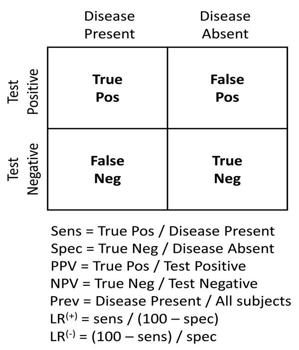 |
Fig. (1). 2x2 box. Disease presence and test results can be simplified into binary choices, resulting in the familiar 2x2 box. Formulae for calculating sensitivity, specificity, and predictive value are shown. The disease prevalence is a population term, referring to the ratio of those with disease to all subjects tested. The analogous term for disease probability in an individual patient is the pre-TP. |
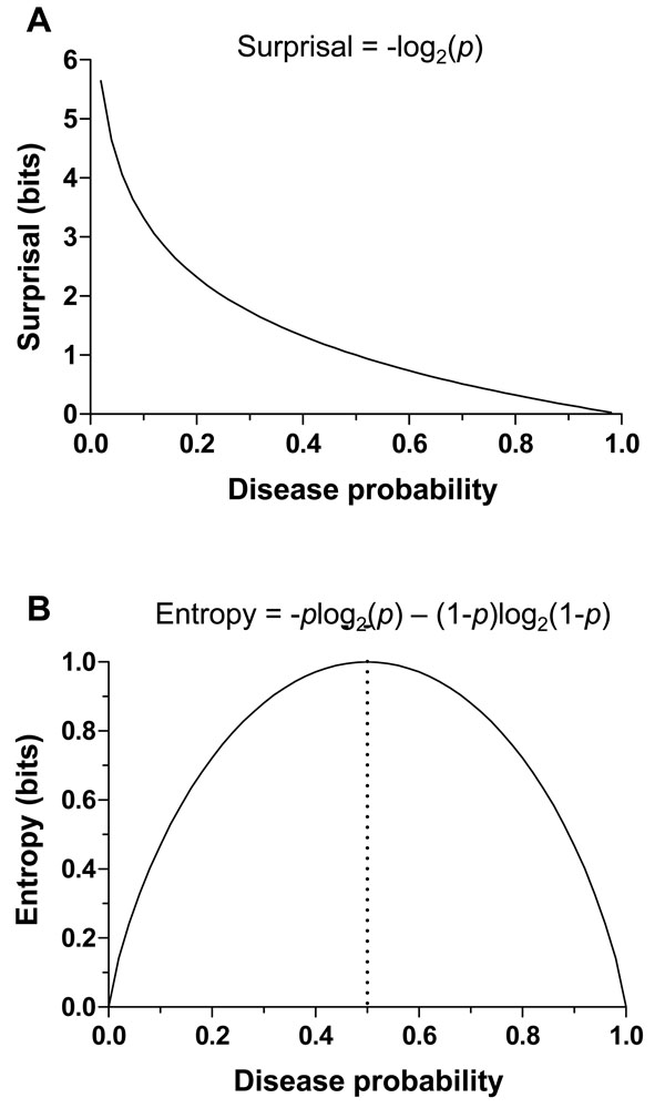 |
Fig. (2). Surprisal and entropy functions. (A) The surprisal function is shown across the probability range from 0 to 1. (B) The binary entropy function for dichotomous disease status is shown across the probability range from 0 to 1. The maximal entropy occurs at p = 0.5 (dotted line). |
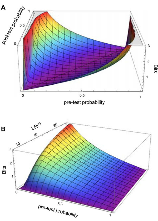 |
Fig. (3). information gain function. (A) The information gain (Z-axis contour) is shown in relation to any given combination of pre-TP (X-axis) and post-TP (Y-axis) values. The information gain is low when the pre-TP and the post-TP are similar to one another (purple “valley”), and high when they are different from one another. (B) Information gain (Z-axis) is shown in relation to combinations of pre-TP (X-axis) and a spectrum of LR(+) values (Y-axis). |
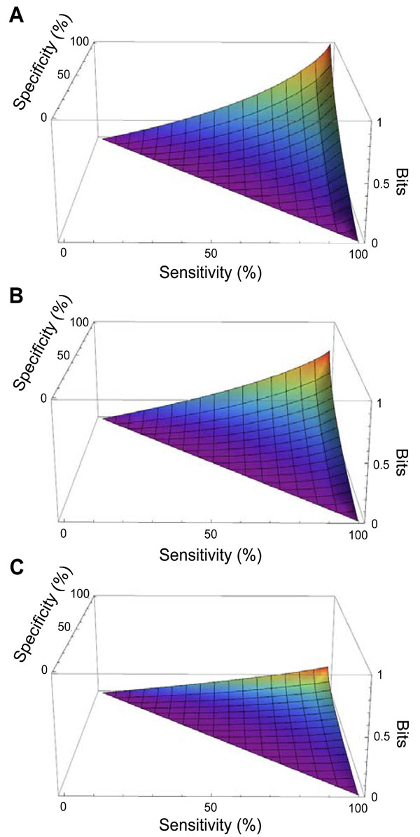 |
Fig. (4). Mutual information function. The mutual information is shown in relation to combinations of sensitivity (X-axis) and specificity (Y-axis), across three pre-TP values: 50% (A), 20% (B) and 5% (C). |
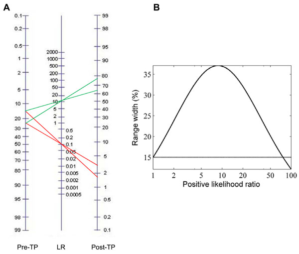 |
Fig. (5). Test results project pre-TP ranges into post-TP ranges. (A) The pre-TP range of 15-25% is projected through a positive and a negative test result using the Bayes nomogram. The positive test result is unexpected (since pre-TP was low), and the resulting post-TP range is expanded (~64-77%). In contrast, the negative test result markedly reduces the probability range, with a post-TP of ~1.5-3%. (B) Starting from a pre-TP range of 15% (horizontal line), the width of the post-TP range at first increases with LR(+), peaks, then decreases and, for strong enough tests, ultimately becomes narrower than the width of the pre-TP range. |
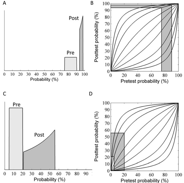 |
Fig. (6). Stretching and warping effects of test results on disease pre-TP distributions. (A) A uniform distribution over the range 75-90% (width = 15%) is transformed by an expected positive test result with LR(+) = 5 into a shifted and warped non-uniform distribution over a narrower range, 94-98% (width = 4%). (B) The reason for the shifting, warping, and range-narrowing is evident from the “football” plot, showing how Bayes’ rule nonlinearly maps pre-test probabilities into post-test probabilities. (C) A uniform distribution over the range 5-20% (width 15%) is transformed by an unexpected positive test result when LR(+) = 10 into a shifted and warped non-uniform distribution over a wider range, 34-71% (width = 37%). (D) Football plot showing the reasons for the shifting, warping, and widening. |
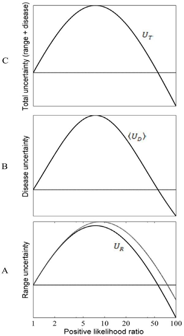 |
Fig. (7). Effects of test results on diagnostic uncertainty.
Uncertainty (entropy) associated with the uniform pre-TP
distribution P from Fig. (6C), plotted as a function of the LR(+).
Values on the y-axes are shown without magnitude to emphasize
the qualitative behavior of these uncertainty measure. The subplots
show: (A) the range uncertainty, UR = H(P) , representing
uncertainty about the pre-TP value; (B) the disease uncertainty,
|
 representing the uncertainty inherent in not
knowing the true disease state uncertainty; and (C) the total
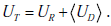
uncertaintyUT , the sum of the other two components
representing the uncertainty inherent in not
knowing the true disease state uncertainty; and (C) the total
uncertaintyUT , the sum of the other two components
 . For the range uncertainty, an additional curve is
shown for comparison (light gray line), representing the entropy for
a distribution with the same width or range as the post-TP
distribution, but with a uniform distribution over this range (rather
than a warped shape).
. For the range uncertainty, an additional curve is
shown for comparison (light gray line), representing the entropy for
a distribution with the same width or range as the post-TP
distribution, but with a uniform distribution over this range (rather
than a warped shape).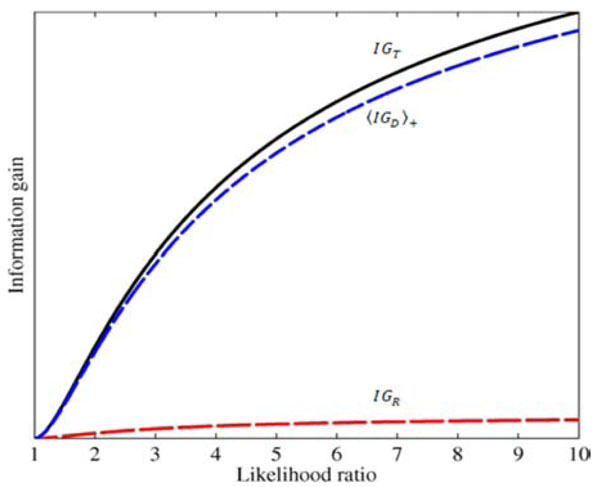 |
Fig. (8). Effects of test results on diagnostic information gain.
The total information gain IGT (solid black curve), and the two
components in the sum |
 , are shown as a function
of the positive likelihood ratio. The range information gain IGR is
the lower red dashed curve, and the disease information gain is the
middle blue dashed curve. These curves are computed using the
distribution over pre-TP values from Fig. (
, are shown as a function
of the positive likelihood ratio. The range information gain IGR is
the lower red dashed curve, and the disease information gain is the
middle blue dashed curve. These curves are computed using the
distribution over pre-TP values from Fig. (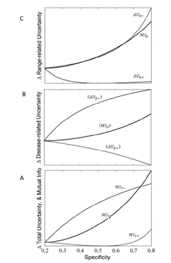 |
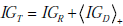
Fig. (9). Mutual information between test results, disease status,
and pre-TP range. (A) Total mutual information MIT and its
components, the mutual information between test results and the
pre-TP range, MIR , and the mutual information between the test
results and disease status, |
 where the brackets indicate the
weighted average over all possible values of the pre-TP. These
three quantities are related by the sum
where the brackets indicate the
weighted average over all possible values of the pre-TP. These
three quantities are related by the sum 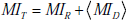 . Each
term can be further broken down into constituents, as illustrated in
B and C. (B) Components of the equation for the disease-state
related mutual information,
. Each
term can be further broken down into constituents, as illustrated in
B and C. (B) Components of the equation for the disease-state
related mutual information,  and
and  , respectively. The disease-state related mutual
information is computed by adding these components together,
weighted by the probability of the corresponding test result,
denoted t+ for a positive result, and t- for a negative test result, i.e.
, respectively. The disease-state related mutual
information is computed by adding these components together,
weighted by the probability of the corresponding test result,
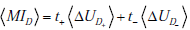
denoted t+ for a positive result, and t- for a negative test result, i.e. 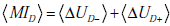 . (C) Components of the equation for the
range-related mutual information, MIR . The comp onent terms are
the change in uncertainty (entropy) that results from positive and
negative test re sults, ΔUR-andΔUR+ , respectively. The mutual
information between the test result and unknown value of the pre-TP (i.e. the range-related mutual information) is computed by
adding these components toget her, weighted by the probabi lity o f
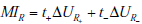
the corresponding test results, i.e. MIR = t+ΔUR+ + t-ΔUR- .
. (C) Components of the equation for the
range-related mutual information, MIR . The comp onent terms are
the change in uncertainty (entropy) that results from positive and
negative test re sults, ΔUR-andΔUR+ , respectively. The mutual
information between the test result and unknown value of the pre-TP (i.e. the range-related mutual information) is computed by
adding these components toget her, weighted by the probabi lity o f
the corresponding test results, i.e. MIR = t+ΔUR+ + t-ΔUR- .The first step in probabilistic (“Bayesian”) interpretation of diagnostic tests is to identify the pre-TP of disease (analogous to the prevalence in the 2x2 box). The next step is to apply the likelihood ratio (LR) value corresponding to the test result. Every test has a positive LR (LR(+)) and a negative LR (LR(-)), both of which are calculated from the sensitivity and specificity of the test as shown in Fig. (1). The LR is used to adjust the disease probability (either by manual calculation, or by nomogram), to yield a post-TP that takes into account all of the relevant information. The resulting post-TP is identical to the predictive value of the test result calculated by the 2x2 box. Thus, the standard 2x2 box and the Bayes nomogram are two ways to arrive at the same information regarding test result interpretation.
In the discussion that follows, we will repeatedly refer to a simple clinical example, the problem of screening and diagnosis of obstructive sleep apnea (OSA). This will illustrate the mathematical concepts and help place them into clinical context.
INFORMATION THEORY: THE SURPRISAL
In this and subsequent sections, we explore how to quantify the information provided by diagnostic test results [13-16]. This exploration will necessitate a framework for handling uncertainty at the level of disease probability, and at the level of ranges instead of point estimates of disease probability. The first essential element in this framework is the information theoretic quantity called the “surprisal”. The term surprisal and its formula are based on the intuitive idea that the less likely an event is to occur, the more surprised we will be if the event is observed. The surprisal is defined mathematically as

INFORMATION THEORY: ENTROPY
We next build upon the concept of surprisal to introduce the concept of entropy and its relationship to uncertainty. Entropy is defined mathematically as the “expected value” of the surprisal, which means the amount on average (over many observations) one will be surprised with regard to an event that may or may not occur. An important feature here, which we will revisit below, is that entropy considers the weighted average of possible outcomes. Thus, the perspective provided by entropy is most meaningful in describing situations before a diagnostic outcome is known, rather than after. This critical point will help translate the concept of entropy into the clinical domain of diagnostic test interpretation, which deals of course with observed test results in individual patients.
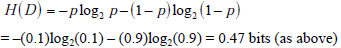
In the simplified framework of the 2x2 box, we are considering only two potential outcomes for health status: disease present (D=1) versus disease absent (D=0), with probabilities g(1) = p , and g(0) = 1- p , where p is the pre-TP of disease. The entropy of disease status, denoted as H(D) , is described in this limited two-outcome case by a simple formula known as the binary entropy function, h(p) . The binary entropy formula is as follows:

Entropy quantifies uncertainty about disease status by considering the average amount of surprise one can expect to have upon learning whether the disease is present or absent, weighted by the probability of each of these possible outcomes. In the above equation, each surprisal term in the average, S( p) = - log2p and S(1- p) = - log2 (1 - p) , is weighted by its probability (p and 1-p, respectively). Like the surprisal, entropy is measured in units of bits.
If the pre-TP of OSA were 20%, the surprise one would have upon ultimately learning that OSA is in fact present by gold standard polysomnography (PSG) is given by the surprisal -log2(0.2) = 2.32 bits, while the surprise one would have if OSA turned out to be absent would be much less (given that the pre-TP is already fairly low): -log2(0.8) = 0.32 bits. The average amount of surprise one will have upon learning the diagnosis, i.e. the entropy, is the weighted average of these two possible outcomes according to the chances of observing each: -(0.2)log2(0.2) - (0.8)log2(0.8) = 0.72 bits.
Before proceeding, we pause to introduce additional elements of notation that will facilitate the discussion of concepts introduced in subsequent sections. Several quantities below will involve taking an average over possibilities, weighting each term in the average according to its probability. The formula for entropy introduced above is one such quantity: it is the average value of the surprisal, S = S(p) , where the averaging is over the two possibilities “disease present”, with probability p, and “disease absent”, with probability 1-p. We denote this average with the following bracket notation:

In some cases discussed subsequently, we require averaging over continuous variables, in which case the bracket notation should be understood as denoting an integral, where each value of the quantity of interest is weighted by a continuous probability distribution.
Although entropy can be calculated at any stage of the diagnostic evaluation, we first consider its application to the pre-TP, before any tests are conducted. As the pre-TP of disease approaches 0 or 1, the associated entropy – or uncertainty – approaches zero. Fig. (2B) illustrates this relationship across pre-TP values from 0 to 1, showing that the entropy approaches zero as the disease probability (p) approaches 0 or 1. The point of maximal entropy occurs when p = 0.5, equally distant from the extreme cases of zero entropy, that is, in the situation in which the patient has a “50-50” chance of having a disease. In this context, the use of entropy as a form of uncertainty is straightforward: one is least uncertain as disease probability approaches 1 or 0, and most uncertain (in this mathematical sense) when disease probability is 0.5.
Note however that the information theoretic meaning of uncertainty refers specifically to event probability, and does not contain any further clinical or semantic meaning. For example, a 50% disease probability may well exceed a clinically defined threshold for initiating treatment, despite diagnostic uncertainty being highest at this point; such a threshold might apply in cases where the treatment is low-risk and/or the risk of failing to treat a true case is high. Certainly OSA falls into such a context – a 50% probability of OSA would at least warrant further testing if not initiation of treatment.
It is also worth noting that the binary entropy function, h(p) quantifies uncertainty only by virtue of how distant the disease probability is from either zero or one, as reflected in the symmetry of the binary entropy function (Fig. 2B). This fact can lead to another apparent paradox, in that a clinically “informative” test result may nevertheless have minimal impact on the degree of entropy or uncertainty, as pointed out by Benish [13-16]. For example, one can imagine a test result moving OSA probability from 10% (low likelihood) to 90% (high likelihood), which might substantially influence clinical management (e.g., treatment with CPAP versus no treatment). Nevertheless, the amount of uncertainty (entropy) associated with 10% and 90% disease probabilities are identical (Fig. 2B). Thus, in order to capture the notion of the amount of information provided a test result (even one that moves disease probability to the mirror symmetric point on the other side of the binary entropy curve), we turn to another information theoretic metric: information gain.
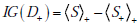
INFORMATION THEORY: INFORMATION GAIN (“RELATIVE ENTROPY”)
The amount of information provided by a particular test result can be described using a quantity known as the relative entropy. Relative entropy is less commonly known as the information gain (IG), which we adopt because it more aptly represents its meaning in the diagnostic setting. Let us suppose that a diagnostic test result for OSA returns positive. Although the OSA disease status remains uncertain, the associated probabilities have been altered. The disease status D initially had probabilities g(1) = p for disease presence and g(0) = 1- p for disease absence. After the test result returns positive, we consider disease status as a new random variable D+ , with the updated probabilities g+ (1) = p+ , for disease presence and g+ (0) = 1- p+ for disease absence; these values can be calculated from the pre-TP and test sensitivity and specificity via Bayes’ rule. The equation for the information gain for a positive test result is defined as:
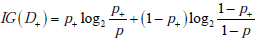
This equation has a structure similar to the entropy formula, with a “probability times log2(probability)” format, but the log probability aspect now refers to the ratio of probabilities: before versus after a test result is obtained. Note also that the first and second terms contain probabilities corresponding to the post-TP and its converse (1-postTP), respectively. The information gain quantifies the difference in the average amount of surprise one has upon ultimately learning the diagnosis before versus after learning about a particular test result. For example, if a positive screening result for OSA raised the patient’s OSA probability from 0.1 to 0.9, we would obtain an information gain as follows: (0.9)log2(0.9/0.1)+(0.1)log2(0.1/0.9) = 2.54 bits.
Using basic properties of logarithms and rearranging terms, we can express this in a more compact and transparent way, using our averaging notation, as
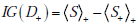
where the ‘+’ subscripts outside the brackets of the  and
and  terms indicate that the weighted average is with respect to the post-TP values of disease status after a positive test result ( p+ and 1- p+) rather than the pre-TP ( p and 1- p ). The ‘+’ subscript inside the term indicates that the surprisal, S , is calculated with respect the post-TP of disease after obtaining a positive test result, p+ , (i.e. S+ = - log2p+), as opposed to the term, in which the surprisal, S , is calculated with respect to the pre-TP, p (i.e. S = - log2p ).
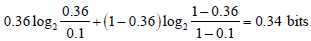
Information gain can also be understood at the population level. Suppose that one is a consultant to whom patients are referred for the possibility of OSA, and that in this patient population one knows that the OSA pre-TP = 10%. The surprise upon ultimately learning the diagnosis in these patients will be -log(0.1) for patients ultimately proven to have OSA, and -log(0.9) for patients ultimately proven not to have OSA. Hence the average amount of surprise one has after diagnosing many of these patients should approach the entropy, H(D) = -(0.1)log2(0.1) - (0.9)log2(0.9) = 0.47 bits. Suppose, however, that more people turn out to have OSA than the pre-TP of OSA would have predicted, specifically, suppose the fraction affected turns out to be 60% in this cohort. This could mean that either the test has a different sensitivity/specificity profile than we believed, or that the prevalence of OSA was higher than we thought. After some investigation, suppose it turns out that in fact the underlying referral pattern was such that we tested only patients who had already had a positive screening test for OSA, and that post-TP = 60%, accounting for the surprisingly enriched disease prevalence we discovered in our referral population. The surprise was initially calibrated to the larger population for whom test results are not known, whereas the actual probability of disease is governed by a different set of probabilities, hence the high average amount of surprise - (0.4)log2(0.1) - (0.6)log2(0.9) = 1.42 bits. Knowing the referral pattern, one can “re-calibrate” ones expectations, and the average amount of surprise will be less now that one knows all the referred patients have positive screening results: -(0.4)log2(0.4) - (0.6)log2(0.6) = 0.97 bits. We can thus define the information gain, IG, comparing our initial expectation versus our later understanding of the biased referral base, as the difference between the average surprisal associated with these two conditions, which is 1.42 - 0.97 = 0.45 bits.
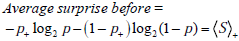
More formally, before we had the extra information, under the mistaken belief that the probability of disease was pre-TP, p, (when in fact in the referral population it was post-TP, p+ ), the average amount of surprise was
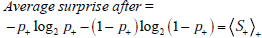
After re-calibration, the probabilities governing one’s amount of surprise and the actual probabilities of disease will match, hence the average amount of surprise will be
Thus the information gain associated with learning the test result is defined as Information Gain = Average surprise before - Average surprise after,
 , as stated above.
Fig. (3A) illustrates the amount of information gain associated with any given combination of pre-TP and post-TP values. The contour surface contains a “valley” with a nadir when the pre-TP and the post-TP are equal – that is, the test result did not alter disease probability (a poor test indeed), and thus provided no information. The peaks occur when the pre-TP and post-TP are most different from one another (low pre-TP to high post-TP, and vice versa). The information gain does of course depend upon observing a particular test result; although not explicitly shown in the plot, one could infer the test result for any given pre-TP and post-TP pair by calculating the appropriate LR value that would provide such a shift in disease probability. Fig. (3B) shows the information gain in terms of pre-TP and LR(+) values, assuming a positive test result is obtained. As expected, the information gain increases as the pre-TP decreases, and is highest when an unexpected result of a strong test occurs: that is, a positive test with high LR(+) in the setting of low pre-TP (or a negative test with low LR(-) in the setting of high pre-TP; not shown).
INFORMATION THEORY: MUTUAL INFORMATION
At this point, we have considered information theoretic terms relevant for interpreting diagnostic outcomes (surprisal and information gain). Information theory also provides a more global context in which to measure how much information, on average, a test result provides about disease status: mutual information. This is the average amount by which uncertainty regarding disease status is reduced by testing in a general sense, without specifying the result obtained in any particular case. Thus, this quantification is more relevant to considering decision support or population-level policies or recommendations in terms of testing. For example, if one were considering OSA screening in a certain population, mutual information can provide some insight into how informative the testing will be overall at the population level.
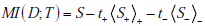
Mutual information explicitly takes into account the pre-TP, test characteristics (sensitivity and specificity), and the different post-TP values after obtaining positive or negative test results. We will need one additional piece of notation to describe the mutual information: Let the outcome of testing be represented by a capital T , a random variable that can be “positive” with probability t+ , and “negative” with probability t-. These probabilities will be specific to the population in which they were measured, that is, they depend on the pre-TP. We can then speak of the mutual information between disease status and test result – in other words, the information about disease status provided by testing, which we denote as MI(D;T ) .
Derivation of Mutual Information
Mutual information is obtained by comparing the entropy associated with the pre-TP of disease and that associated with the probability of disease given a test result. Drawing from the equations above, we can calculate the mutual information in two steps. First, we obtain the uncertainty associated with the disease status, D , before testing (with probabilities g(1) = p and g(0) = 1- p ), which is equal to

Second, we obtain the uncertainty associated with the disease status after a positive result, D+ , which is expressed using the probabilities g+ (1) = p+ , (i.e., the post-TP) and g+ (0) = 1- p+ . Thus, the entropy of D+ is written as

The first term is the surprisal upon finding that a patient with a positive result actually has the disease, weighted by the probability of that outcome (ie, the post-TP), p+ . The second term is the surprisal upon finding that a patient with a positive result actually does not have the disease, weighted by the probability of that outcome (ie, the 1-post-TP), 1- p+ . Together, they comprise the average surprisal associated with a positive test result, .
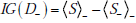
The disease status after a negative result is D-, based on the probabilities g- (1) = p- ,(i.e., the negative predictive value) and g- (0) = 1- p- ; these probabilities can be calculated by Bayes’ theorem, or by the 2x2 box, equivalently. The entropy associated with D_ is written as

To express the average entropy, we weight each of these terms by the probability of their associated results, i.e. the probability of a positive (t+) or negative (t-) test result. The difference between the first of these (pre-test entropy) and the weighted combination of these last two entropy values (post-test entropies) is the mutual information, that is

Alternative Formulae for Mutual Information
It is instructive to express the formula for mutual information in several different ways. First, using the fact that  and denoting the change in uncertainty due to a positive or negative test result as
 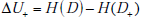 and
and 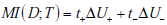 , we can rewrite the mutual information simply as the average change in the amount of uncertainty, where the average is simply the sum of the changes in uncertainty due to a positive and negative test results, weighted by the probability of those results,
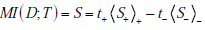
Alternatively, for more direct comparison with the formula for information gain, we can also express this formula directly in terms of average surprisal values
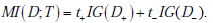
Finally, it is also possible (see Appendix A) to express mutual information as simply the average information gain associated with testing (i.e. averaging over a large population, or, for individuals, the “expected” information gain, with the information gain associated with positive or negative test results weighted by their probabilities):
Illustrations of Mutual Information
Fig. (4) shows the mutual information provided by diagnostic tests with any combination of sensitivity and specificity, in the setting of three representative pre-TP values (5%, 20%, 50%). As expected from the symmetry of the binary entropy function, h(p) , the mutual information for any of these hypothetical tests is greatest when the pre-TP is 50%. The plots for pre-TP values of 80% and 95% are identical to those for pre-TP values of 20% and 5%, respectively, due to the symmetry seen in Fig. (2B) (not shown). For any given pre-TP, the mutual information increases as sensitivity and specificity increase, as expected.
To summarize, the critical distinction between the mutual information and the information gain is that both possible outcomes of the dichotomous test result are included in the mutual information calculation. Mutual information can be thought of as a metric of overall test performance, based on the combination of test characteristics (sensitivity and specificity) and the clinical context provided by the pre-TP of disease. The information gain, by contrast, considers the surprise at ultimately learning the diagnosis if one does versus does not know a particular test result. The clinician managing an individual patient must, of course, act on the specific test result in hand, and not on the spectrum of possible outcomes of testing. Nonetheless, the mutual information provides important insight into test performance, on average, in a given population, which may be useful when comparing tests, or when making policy-level decisions about diagnostic testing.
SUMMARY OF OSA DIAGNOSIS EXAMPLE OVER SEVERAL INFORMATION THEORY METRICS
To demonstrate the logic and application of these information theoretic quantities, consider a hypothetical screening test for which sensitivity = 90% and specificity = 82% (much better than the current best-performing OSA screen, the STOP-BANG questionnaire), performed on a patient who has a pre-TP of OSA = 10%. From the pre-TP estimate, we can calculate the surprisal of an event with probability = 0.1, which is -log2(0.1), or 3.32 bits. From the sensitivity and specificity, we can calculate the LR(+) and LR(-) values of 5 and 0.12, respectively, for this screening test. Using Bayes theorem (or the nomogram), we can determine that the probability of OSA given a positive test result is 35.7% and the probability of OSA given a negative test result is 1.4%.
From these post-TP values, we can calculate two values of information gain, one for the case of a positive test result
and one for the case of a negative test result
The different numbers of bits in the information gain for these results suggests that more information was contained in the unexpected, positive test result. This reflects and quantifies the fact that the positive result caused a greater absolute change in OSA probability (10% to 36%, a 26% absolute difference), compared to the negative test result (10% to 1%, a 9% absolute difference).
Next, the mutual information informs us about overall test performance (for example, across a population of patients), or how much information the test will provide on average. We will calculate it using the first of the formulae for mutual information that we introduces above, i.e. : . .
.
It is easiest to break this calculation into steps. First, calculate the pre-test uncertainty
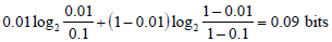
Next, calculate the uncertainty after a positive test result, H(D+ ) , by using the post-TP after a positive result, 0.36, according to: -(0.36)log2(0.36) - (0.64)log2(0.64) = 0.94 bits. We then multiply this uncertainty by the probability of a positive test, t+ . This value, t+ , is calculated by knowing the sensitivity, specificity, and pre-TP, as follows. The probability of a positive result given disease is the sensitivity, while that of positive result given no OSA is 1-specificity. Each of these is weighted according to the prior, such that: sensitivity x pre-TP + (1-specificity) x (1-pre-TP) = the probability of a positive test result. Using our example, we have 0.1·0.9 + 0.9 ·0.18 = 0.25 = t+ . Third, calculate the uncertainty after a negative test result, H(D- ), using the post-TP after a negative result, 0.02, according to: -(0.01)log2(0.01) - (0.99)log2(0.99) = 0.10 bits. We weight this by the probability of obtaining a negative test result, t- , which we can get by simply subtracting 1-t+, that is, t- = 0.75 . Finally, putting all the pieces together, we have MI (D;T ) = 0.47 - (0.25·0.94) - (0.75·0.1) = 0.16 bits.
UNCERTAINTY WHEN A RANGE OF PRE-TP VALUES IS GIVEN: BAYESIAN APPROACH
We have until now considered only point estimates of pre-TP for convenience. However, in cases of clinical judgment and epidemiological studies alike, the pre-TP may be arguably better represented by a range of plausible values. In this and subsequent sections, we investigate the impact of ranges (instead of point estimates) of pre-TP on the resulting post-TP. Initially, we consider these ranges simply as boundaries of possible values, without specifying any particular distribution over this range (we will address this later). Thus we consider a given uncertainty interval (say, 20±5%) for the pre-TP of disease (Fig. 5A). Using any given combination of sensitivity and specificity values, we can implement Bayes’ theorem to generate a post-TP range. In the nomogram, note that the 20±5% range becomes ~30% larger in the projected post-TP range (~64-77%) when the result of a test with LR(+) of 10 is unexpectedly positive, while it shrinks markedly when the test result was negative (and therefore expected given the low pre-TP). Fig. (5B) shows the relationship, over a broad range of LR(+), between the pre-TP range (assumed to be 15% in the figure, indicated by the horizontal line), and post-test probability range. We see that the width initially grows, then at extreme LR(+) values (corresponding to very “strong” test results), the width again shrinks. We will have more to say about this fact below.
These plots also provide an opportunity to preview the question of whether uncertainty, considered in quantitative (i.e. information theoretic) terms, increases due to an unexpected test result. Clearly the range of possible disease probabilities has grown in absolute terms for a particular patient’s positive result (or shrinks if the result was negative). We might therefore expect that uncertainty (measured in information theoretic terms) should increase in response to an unexpected result, and we will see below that this is indeed the case. On the other hand, the weighted average of the post-TP ranges after a positive versus a negative test result would be smaller than the pre-TP range, hence performing the test can be considered to decrease uncertainty about the disease status on average, even though some of the time, the result will be unexpected and increase uncertainty. This leads us to expect that testing reduces uncertainty on average, which we will see is also the case.
Interlude: Simplifying the Notation
In introducing the information theoretic concepts appropriate for quantifying the impact of test results on diagnostic uncertainty, we have introduced several different notational conventions. While these have been useful in conveying the concepts thus far, in the section that follows it will be helpful to introduce a few shorthand notations for the three main information theoretic quantities of entropy, information gain, and mutual information. The reason for doing this is that concepts in the final sections build upon those in previous sections, and without simpler shorthand for the core building block concepts the notation becomes cumbersome. From here on, we will use the following: Entropy, or uncertainty, will be denoted U ; information gain, IG ; and mutual information, MI. Thus far all of these quantities have referred directly to the uncertainty of information associated with disease status, as opposed to the uncertainty associated with estimates of the pre-TP itself. We will thus distinguish, using subscripts, between quantities directly concerned with disease status, and those associated with the range of pre-TP, as follows: The disease-status uncertainty is UD , information gain (about disease status) for positive test is IGD , and the mutual information (between disease status and test results) is MID . These are the quantities described above, for which we have already presented formulas. By contrast, the corresponding quantities associated with the range of pre-TP values (introduced below), will be denoted by UR , IGR , and MIR .
UNCERTAINTY WHEN A RANGE OF PRE-TP VALUES IS GIVEN: INFORMATION THEORETIC APPROACH
We have seen how the range of pre-TP values can be transformed via Bayes’ rule into an expanded post-TP range, due to an unexpected test result. We now quantify this effect in information theoretic terms, relating changes in the post-TP range to changes in uncertainty. To do this we need to characterize the two sources of uncertainty under discussion:
- Uncertainty regarding the pre-TP, p. As mentioned in the introduction, one way to think about pre-TP uncertainty is to consider it a random variable, P , that can take on values within a range, instead of a point estimate. That is, for the pre-TP, p , we specify that it falls within a range, a ≤ p ≤ b . We can be even more explicit by considering how probable each value is, that is, by specifying a distribution of pre-TP values over the range. This can be formalized by specifying a function, f (p) , denoting the probability that pre-TP assumes any particular value p within the specified range. For simplicity, we will first assume a uniform distribution, that is, all probabilities within the range are equally likely, so that f ( p) = 1/ (b-a) within the range, and f ( p) = 0 outside the range. For concreteness, referring back to OSA example, suppose that rather than knowing that the pre-TP is precisely 10%, we know only that the pre-TP value lies in the range 5-20%, with no reason to consider any of these values more likely than any other (as in Fig. 6C). The uncertainty associated with not knowing the pre-TP value precisely is then UR .
- Uncertainty regarding disease status, UD . For any given pre-TP value the disease status is uncertain (except at the extremes, pre-TP = 0 or 1). We can represent this as before by thinking of the disease status as a random variable, D , that can assume the value of 1 (disease present) or 0 (disease absent).
In our OSA example, the disease-status uncertainty UD is precisely the source of uncertainty we have focused on up to this point, i.e. our uncertainty about whether our patient has OSA.
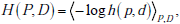
However, we see that now the disease probabilities depend on an unknown value for the pre-TP (i.e. on the random variable P ), making the expression for the uncertainty of this value slightly more complicated. It turns out that the needed expression can be derived easily after first specifying the joint probability distribution of the disease state with that for the pre-TP value. We denote this joint distribution as h(p,d) . Using Bayes’ rule, we write h( p,d) = f ( p)g(d | p) . This formula reads as follows: the entropy associated with the disease status and the pre-TP range is a function of the probability distribution over the range, times the probability of disease given this range. Thus, the probability of disease (D = 1) or disease absence ( D = 0 ) when the pre-TP is equal to p is given by g(1|p) = p or g(0|p) = 1- p , respectively.
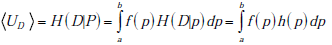
From these building blocks, it follows that the total uncertainty regarding disease status before any test is performed is given by the combination of the entropy associated with the two random variables, P and D . This joint entropy is written as H(P,D) , and it can be broken into a sum of two terms, H (P,D) = H (P) + H(D | P) (see Appendix B). Hereafter, we will refer to UR = H(P) as the `range uncertainty’, and UD = H (D|p) as the `disease uncertainty’. The UR = H(P) term is the uncertainty (entropy) regarding the pre-TP. The 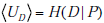 term is the uncertainty regarding the disease probability averaged over the range of possible pre-TP values under consideration (that is, each point in the range contributes to the average, weighted by its probability). Their sum, the `total uncertainty’, is written as H(P,D) . The total uncertainty can now be compactly expressed as
In our OSA example, our total uncertainty is composed of our uncertainty regarding the true value of the pre-TP of disease, and our uncertainty regarding the patient’s disease status.
Range Uncertainty: How a Test Result Warps the Distribution of Pretest Probabilities
As discussed above, updating disease probability when the pre-TP was considered as a range instead of a point estimate involves a change in the width of the range. However the shape of the probability distribution over the stretched range also changes, owing to the nonlinearity of Bayes’ formula. As an example, suppose the pre-TP is uniformly distributed over the range 75-90% (width = 15%, Fig. 6A “pre”). In this case of high pre-TP, if a positive test result is observed, we find that the post-TP range is narrower than the pre-TP range: 94-98% (width = 4%, Fig. 6A “post”). This is intuitive, as the positive result was expected (the pre-TP was high to begin with), and thus we would expect our uncertainty to decrease, which it did (smaller range in post-TP). However, in addition to this narrowing effect, we see that the shape of the distribution over the post-TP is no longer uniform. Rather, the distribution is shifted so that the bulk of the probability `mass’ is concentrated toward the right side of the distribution. Fig. (6C) shows the consequences an unexpected positive result, obtained when the pre-TP was low: 5-20% (width 15%, Fig. 6C “pre”). Given an LR(+) value of 5 for the positive test result, the post-TP range stretches to 21-56% (width = 35%, Fig. 6C “post”), and the probability distribution is shifted toward the right-most border of the range.
While we can appreciate the widening of the post-TP range relative to the pre-TP range using the Bayes’ nomogram as described earlier, to understand the alteration of the pre-TP distribution’s shape it is helpful to examine the nonlinear mapping from pre- to post-TP more explicitly. Consider the `football’-shaped plot of Fig. (6B), in which the curved lines correspond to different LR values. Curves below the straight diagonal line (LR=1) correspond to negative test results (i.e., when LR < 1), and the curves above it correspond to positive test results (i.e., when LR > 1). For the example shown in Fig. (6B, D), LR(+) = 5. Note that curves for LR > 1 have a steep initial slope at lower pre-TP values, which progressively decreases with increasing pre-TP. This shape explains the shift in probability distribution mass seen above. Given the concave downward shape of the LR>1 lines, for any two ranges of equal width on the pre-TP axis (that is, any two ranges that contain equal amounts of probability mass), the right-most one will be mapped through a more shallowly sloped portion of the LR curve. Mapping through a more shallow portion translates into a more narrow portion of the post-TP axis. This explains the concentration of pre-TP distribution toward higher post-TP values in our example.
We will use the case illustrated in Fig. (6C) (pre-TP estimated to lie in the interval 5-20%, a diagnostic test with LR(+)=5, LR(-)=0.12) to continue our running OSA example, treating this range as a clinician’s estimate of the pre-TP that a particular patient has OSA, as might be the case for a patient who has some typical signs (e.g. excessive daytime sleepiness) but not others (not obese, no snoring). A positive test for OSA in such a patient produces considerable alteration of the pre-TP of disease. After the positive test, the quantitatively-inclined clinician will be left thinking that the patient may or may not have OSA (as quantified by the distribution of the post-TP values), with the majority of the probability mass now concentrated near the middle of the zero-to-one range, i.e. a state of much-increased uncertainty. We now turn to quantifying this uncertainty numerically, paralleling our earlier discussion when the pre-TP value was known precisely.
Range Uncertainty: Quantifying the Effect of Distribution Widening and Warping on Uncertainty
Analogous to the formula for uncertainty (entropy) regarding disease status, the expression for the range uncertainty H(P) is given by adding up the value of the surprisal function S(p) over the range of possible values a ≤ p ≤ b , weighting each term in the sum by the corresponding probability, f (p) . However, in this case we have a continuous range of possible pre-TP values, so `adding up’ really means computing an integral,
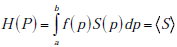
Recall that the angled brackets indicate averaging with respect to a continuous distribution f (p) rather than a discrete (i.e. binary) probability distribution. In Fig. (7A), the value of the entropy associated with the uniform pre-TP distribution of the ‘unexpected positive result’ example (from Fig. 6C, “pre”) is plotted as a solid straight line, to allow comparison with the post-TP range entropy, shown as a solid black curve. For comparison, a lighter gray line represents the entropy that would result if the distribution over disease probabilities in the post-TP setting merely increased in width, while remaining uniform (rather than being warped, as is actually the case). This illustrates the intuitive fact that for any two probability distributions over the same range of values, a uniform distribution represents the situation of greatest uncertainty (in other words, the least amount of structure of the probability distribution). Nevertheless, we see that the dominant effect on the post-TP range uncertainty in this example results from the change in the width (rather than the shape) of the distribution. For most of the LR values shown, the post-test range uncertainty line is above the pre-test range uncertainty line, in agreement with the intuition that a wider probability range entails greater uncertainty. However, for very large LR(+) values, the range uncertainty again decreases, corresponding to the fact that the width of the post-TP distribution shrinks relative to the pre-TP range for high LR values (compare with Fig. 5B). The reason for this can be appreciated by considering again the football plots in Fig. (6B, D): The LR curve for large LR(+) tests approaches the upper left corner of the plot, hence projecting pre-TP ranges to such LR curves will encounter the shallow portion, and thus project the pre-TP range to a narrower post-TP range.
In the OSA example, where LR(+)=5, and the endpoints of the range were a=5%, b=20%, the same values were used in Fig. (6C) and in computing the curves in Fig. (7). In this case, the distance between the dotted line (pre-TP uncertainty) and the solid curve (post-TP uncertainty) represents the effect of widening, shifting and warping of the range uncertainty induced by a positive OSA test result. Specifically, the positive result increased the range uncertainty by 1.17 bits.
Disease Uncertainty
For any given value of the pre-TP p, the disease uncertainty UD = H (D|p) is simply given by the binary entropy function h( p) = - p log2p - (1- p) log2 (1 - p) . The average uncertainty UD = H(D | P) in the expression above is thus simply the average value of the binary entropy function over the range of pre-test probabilities, i.e.
The pre-test disease uncertainty for the case we have been considering (uniform distribution of pre-TP over the range 5-20%, Fig. 6C) is plotted as a solid horizontal line in Fig. (7B). The curve of post-test disease uncertainty versus LR shown in Fig. (7B) has a qualitatively similar shape to the curve for the post-test range uncertainty. The reason is essentially the same as in the situation with unexpected results when we were considering single values for the pre-TP rather than a range: Disease uncertainty (entropy) is highest when the probability of disease is 50%. Hence, we see that for intermediate LR values (greater than 1, but not `too’ large, as in Fig. 6C, “post”), the post-TP values are distributed in such a way that values near to 50% are more likely than in the pre-test setting, causing the post-test disease uncertainty to be greater than the pre-test disease uncertainty. Nevertheless, as we have seen, for very large LR(+) values, a positive test result causes the post-test disease probabilities to become narrowly concentrated around a high post-TP (as in Fig. 6A, “post”), far from 50%, hence the post-test disease probability decreases for large LR(+) values.
From the OSA example in which LR(+)=5, a positive result in this setting of an uncertain pre-TP value produces an increase in the disease uncertainty by 0.41 bits (the distance in bits between the dotted line and the overlying curve).
Total Uncertainty
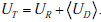
As mentioned above, the total uncertainty UT = H(P | D) is the sum of the range uncertainty UP = H(P) and disease uncertainty, . Clearly, given the similar overall shapes of the curves for these component parts of the sum, the overall shape of the curve for the total uncertainty shows the same behavior: increased uncertainty for low and intermediate LR values, followed by decreased total uncertainty in the face of unexpected but highly compelling (high LR(+)) positive test results (Fig. 7C).
Once again, for our OSA example, this means that the total increase in uncertainty associated with a positive test result is composed of the 1.17 bits contribution from the increased range uncertainty, plus the 0.41 bits contribution from the increase in the disease uncertainty, for a total increase in uncertainty of 1.58 bits.
INFORMATION GAIN WHEN A RANGE OF PRE-TP VALUES IS GIVEN
We can also extend the notion of information gain to handle pre-TP values given as a range rather than as a simple point estimate. Using notation from the previous section, when we obtain a positive test result, we effectively update the random variables representing the range of pre-TP and disease status, P,D , to obtain new random variables P+ ,D+ (assuming a positive test result). These new random variables clearly have new probability distributions, i.e. a positive test result effectively causes the following transformation to take place: h( p,d) = f ( p)g(d|p) → h+ ( p,d) = f+ ( p)g+ (d|p), where the “+” subscript indicates the transformation of the pre-TP distribution f (p) by the positive result into its “warped” counterpart f+ (p) , as illustrated previously in (Fig. 6A, C). Similarly, we express the transformation of the pre-TP g(d | p) into the post-TP as g+ (d | p) . As with the expression for uncertainty, the information gain incurred by a positive test result can be naturally expressed as a sum of two terms
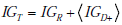
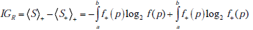
In this sum, the first term, IGR , represents the information gain related to the transformation of the distribution of probabilities over the range of possible pre-TP into the shifted and warped distribution over the range of possible post-TP (i.e. the transformation f ( p)→ f+ ( p) , namely
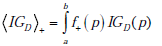
The second term, IGD , represents the information gain associated with the update of any given pre-TP into the corresponding pos-TP (i.e. the transformation g(d|p)→g+ (d | p) , averaged over the entire range of possible disease probabilities, i.e. IGD = IG(D+ ) , as defined previously, which is in fact a function of the pre-TP, p, so that we can write IGD = IGD (p) , and
An illustrative example is shown in Fig. (8), plotting information gain against LR(+), and assuming as before that the pre-TP value is uniformly distributed between 5-20% (as in Fig. 6C). In the figure, the red and blue lines represent the first and second terms, IGR , and  , respectively, and the black line represents their sum, i.e. the total information gain, IGT . Notice that information gain is always positive, despite the observation in the previous section that, for a wide range of LR values the amount of uncertainty increases. While this may seem paradoxical (at least semantically), it actually makes sense if we recall that information gain is a measure of the discrepancy between two probabilistic models. In this case, we treat the post-test situation, modeled by h+ ( p,d) = f+ ( p)g+ (d | p) , as the most “up-to-date” model, being informed by the positive test result now in-hand. The information gain then tells us how big was the discrepancy between this and the pre-test model, h( p,d) = f ( p)g(d | p) , thus, how much information was “gained” in updating the pretest model.
In our OSA testing example (LR(+)=5), the total information gain resulting from a positive test in this setting of an uncertain pre-TP is 0.09 bits. This total is composed of a gain of 0.004 bits related to the gain of information about the pre-TP value, and 0.0986 bits related to the disease status.
MUTUAL INFORMATION WHEN A RANGE OF PRE-TP VALUES IS GIVEN
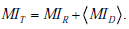
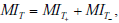
Finally, we can extend the concept of mutual information introduced earlier to the situation in which a range of pre-TP values is given. Not surprisingly, this total mutual information can be expressed as a sum of two terms
Here, MIR describes the average amount by which a test result decreases the overall uncertainty associated with the distribution over disease probabilities, by narrowing and/or reshaping the distribution. The term  is the amount of uncertainty reduction conferred by a test result for any given pre-TP p , averaged over the range of possible pre-TP within the allowed range.
To apply this formula to our OSA testing example, consider the population level viewpoint in which our knowledge of the pre-TP value for the population is uncertain, modeled by the distribution in Fig. (6C). From here, let us ask how much information we may gain, on average over this population, by performing the hypothetical OSA test above, with LR(+)=5, LR(-) = 0.12 (i.e., sensitivity 0.92, specificity 0.8). The relevant calculations yield a mutual information value between the average testing outcome and the pre-TP value, IR , or 0.1827 bits; we also obtain a disease-status mutual information of 0.1747 bits, for a total mutual information of 0.3574 bits.
It is important to note that the overall mutual information and its constituent terms are always positive quantities, i.e. the average effect of testing is to provide a net decrease in uncertainty, despite the fact that individual positive or negative test results may either increase or decrease uncertainty. This point can be better understood by further dissecting each term in the total mutual information MIT into its constituent parts
where t+ and t- represent the probability of obtaining positive and negative test results, respectively. Thus, each term contributing to the total mutual information is in turn a sum of a “positive” and “negative” component, i.e. a component expressing the change in uncertainty incurred by a positive test result, weighted by the probability of a positive test result, and a complementary term for negative test results. Substituting these expressions for the terms in the previous expression for the total mutual information and rearranging, we see that the total mutual information can be re-expressed as a sum of “positive” and “negative” test result components:
with  . As discussed in our initial presentation of mutual information, for any useful test (one that alters the probability of disease), the average result will be to decrease overall uncertainty. This is true despite the fact that uncertainty increases in cases of unexpected test results, because these are less likely compared to the more probable expected results, which receive more weight in the above expressions. Hence, mutual information is always positive. The relationships just described are illustrated in Fig. (9).
Calculating these quantities for our OSA example, we find a value for the positive component of MIT+ = 0.0806 bits, and for the negative component MIT- = 0.2768 bits, for a total average quantity of information obtained by testing of 0.3574 bits, identical to the value arrived at by alternative means above.
DISCUSSION
Rational diagnostic test interpretation requires considering the combination of 1) test performance in discriminating disease presence from absence, and 2) the baseline probability of disease before any testing is undertaken. In the most simplified formulation, the test result and the disease status are considered to be dichotomous, allowing the familiar terms of sensitivity and specificity and disease probability to be employed. Whether one considers the Bayes’ nomogram, or uses the 2x2 box, the post-TP of disease given a test result can be assessed in a straightforward manner by considering sensitivity, specificity and pre-TP values.
Here, we have provided parallel approaches using information theoretic concepts. We see that an information theoretic formulation provides insight into diagnostic test interpretation at the level of specific test results in specific patients (through the constructs of surprisal and information gain), as well as in a more general or population sense that considers the weighted average of testing outcomes within a populations (through the constructs of entropy and mutual information). Like the concept of uncertainty, the concept of information can take on various meanings depending on the context. We have striven to clarify the technical meanings of these terms and concepts, and to point out how these relate to and differ from their usual senses in the medical vernacular, in hopes that an appreciation of the semantic variability of these terms may help distinguish the clinical parlance from the information theoretic meaning of these terms.
Uncertainty in the interpretation of test results assumes at least two key forms- one form relating to the fact that considering disease status as a probability in itself expresses a degree of uncertainty, and another form relating to need to estimate the disease probability as a range of possible values rather than as a single, precise number (e.g. the confidence interval of a pre-TP estimate). This latter form of uncertainty, implicit in the typical unavailability of precise disease probability estimates, contains certain non-intuitive features, as described here and previously [19]. The vagaries and diversity of patient presentations (which form the basis of pre-TP estimations) suggest that the pre-TP may be represented better by ranges (more precisely, distributions over ranges) rather than by simple point estimates. In this paper we have provided the first deomonstration of how this additional uncertainty regarding pre-TP estimates can be rigorously quantified using appropriate concepts from information theory.
CONFLICT OF INTEREST
The authors confirm that this article content has no conflicts of interest.
NOTES
1 Simon Parsons, Qualitative methods for reasoning under uncertainty, 2001, MIT Press.
ACKNOWLEDGEMENTS
Dr. Bianchi receives funding from the Department of Neurology, Massachusetts General Hospital, and the Center for Integration of Medicine and Innovative Technology. MBW and SSC are partially supported in this work by NINDS-NS062092.
APPENDICES
Appendix A: Derivation of Mutual Information as Expected Information Gain
Here we show that the mutual information between the disease state and a diagnostic test result can be expressed as the expected information gain, i.e. MI (D;T ) = t+IG (D+ ) + t-IG(D- ) , where t+ and t- are the probabilities of positive and negative test results, respectively. Recall from the main text that the one expression for the mutual information is
whereas an expression for the information gain from a positive test result is
and for a negative test result
Noting that t+ + t- = 1 , then adding and subtracting the terms S+ and S- in the appropriate places thus yields

Hence, we need only to show that the first three terms sum to zero. For convenience, we use the overbar notation to denote the converse of a probability,  . We then have, for the sum of the first three terms,

Recall that p+ = Pr(D+ |T +) , and t+ = Pr(T +) , so by Bayes’ rule p+t+ = Pr(D+ ,T+ ) . Similarly, p- = Pr(D+ |T -) , and t- = Pr(T _) , hence p-t- = Pr(D+,T -) . Thus the sum

so that consequently, the first term vanishes. Similar calculations show that the second term also vanishes, proving the desired result.
Appendix B: Derivation of the Decomposition Formula for Joint Entropy
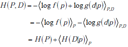
Here we show that the joint entropy of two random variables can be written as the sum of the entropy of the distribution for the first random variable plus the entropy of the distribution for he second random variable conditional on the first, i.e. H (P,D) = H (P) + H (D|P) . This follows directly from the definition of entropy and from Bayes rule. Using the notation from the main text, we write the joint distribution as h( p,d) = f ( p)g(d|p) , which is simply an expression of Bayes’ rule, or equivalently, the definition of conditional probability. Then, using our bracket notation to denote averaging, we have
 where the subscripts indicate performing the weighted averaging over the entire range of both random variables P and D . Substituting and using the basic property of logarithms that log x · y = log x + log y , we have
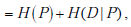
as was to be shown.