RESEARCH ARTICLE
Region Quad-Tree Decomposition Based Edge Detection for Medical Images
Sumeet Dua*, Naveen Kandiraju, Pradeep Chowriappa
Article Information
Identifiers and Pagination:
Year: 2010Volume: 4
First Page: 50
Last Page: 57
Publisher Id: TOMINFOJ-4-50
DOI: 10.2174/1874431101004020050
Article History:
Received Date: 10/10/2009Revision Received Date: 15/11/2009
Acceptance Date: 15/11/2009
Electronic publication date: 28/5/2010
Collection year: 2010
open-access license: This is an open access article licensed under the terms of the Creative Commons Attribution Non-Commercial License (http://creativecommons.org/licenses/by-nc/3.0/) which permits unrestricted, non-commercial use, distribution and reproduction in any medium, provided the work is properly cited.
Abstract
Edge detection in medical images has generated significant interest in the medical informatics community, especially in recent years. With the advent of imaging technology in biomedical and clinical domains, the growth in medical digital images has exceeded our capacity to analyze and store them for efficient representation and retrieval, especially for data mining applications. Medical decision support applications frequently demand the ability to identify and locate sharp discontinuities in an image for feature extraction and interpretation of image content, which can then be exploited for decision support analysis. However, due to the inherent high dimensional nature of the image content and the presence of ill-defined edges, edge detection using classical procedures is difficult, if not impossible, for sensitive and specific medical informatics-based discovery. In this paper, we propose a new edge detection technique based on the regional recursive hierarchical decomposition using quadtree and post-filtration of edges using a finite difference operator. We show that in medical images of common origin, focal and/or penumbral blurred edges can be characterized by an estimable intensity gradient. This gradient can further be used for dismissing false alarms. A detailed validation and comparison with related works on diabetic retinopathy images and CT scan images show that the proposed approach is efficient and accurate.
1. INTRODUCTION AND BACKGROUND
In computer vision and image processing, the boundaries of object surfaces often lead to oriented-localized changes in the intensity of the image, called edges. This observation combined with edge detection as the initial step in image segmentation-based learning methods, has fueled a long search for a good edge detection algorithm to use in image processing [1]. In edge detection, significant variations of the grey-level image are localized, and the physical phenomena that originated them are identified. This process is important, and has varied applications in object recognition, image enhancement, and content-based image retrieval (CBIR) application domain areas.
Edge detection techniques transform images to edge images exploiting the changes of grey tones in the images. The changes may constitute changes in the boundaries of an object; markings on an object that show a sudden discontinuity or a considerable difference in the intensities between the neighboring pixels are considered edges. As a result of this transformation, the edge image obtained contains edges that exist without causing any changes in the physical qualities of the inner portions of the image. This property is significant for several medical informatics applications [2]. Since edges correspond to variations in several properties, different types of edges might occur in an image. The most common types of such edges are step edges, line edges, and junctions [3, 4]. Step edges are the most common type of edges that occur in medical images, and they are the first order discontinuities in an image.
The method proposed in this paper performs region quadtree decomposition of an image [5]. Quadtree is a spatial data structure used to represent a region, which, in turn, can be represented by means of its interior or by means of its boundaries [6]. Based on the hierarchical decomposition, the region quadtree of a bounded image divides an array into four equal sized quadrants [7]. See Fig. (1) for an illustration of the region quadtree decomposition.
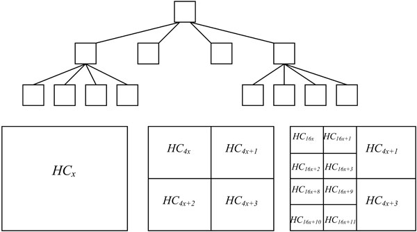 |
Fig. (1). The coverage of a quad tree. |
Assuming the size of the input image array is m x n. Without the loss of generality, we assume m and n are powers of two. If a covering quadtree represents an entire array, its four children represent the four quadrants of the array, and each quadrant is recursively subdivided in the same manner and represented by corresponding children at successively deeper levels of the quadtree. Our goal is to identify the quadtree subtree with B leaves, such that the partitioning of the array induced by this tree yields homogeneous leaves [8].
In the case of a binary scale image, the condition of homogeneity defines all the pixels within the block as either a 1 or a 0. Since we work with medical images that are based on the gray-scale, we define a homogeneity condition (HC). HC is the difference between the least pixel intensity and highest pixel intensity within a node of the quadtree and should be less than a threshold (τ). This requirement means that the decomposition is performed until no two pixels within the blocks obtained differ by an intensity value greater than the threshold.
Note that each node x in a quadtree represents a 2l x 2l square for some integer l. Each such node has two disjoint 2l x 2l-1 sized left and right-half rectangles, denoted l and r, respectively. Each rectangle of that form has two disjoint 2l-1 x 2l-1 sized top and bottom squares, denoted t and b, respectively. Thus, each square x of size 2l x 2l has four disjoint 2l-1 x 2l-1 squares, which are denoted by tl, tr, bl, and br in clockwise order starting with the top-left quadrant of x (see Fig. 2). The height of the left nodes is 0; the height of the left node parents is 1, and so on.
 |
Fig. (2). Partitioning a node for recursive definition. Leftmost square: height = i+1. Rightmost square: Height = i. |
For our experiment, we consider any node x, and define HCx(i) to be the difference between intensities of the node x, partitioned into i blocks as per the quadtree partitioning. Then we have
 |
(1) |
Here,  is the minimum intensity in the left rectangle of the node at x with i blocks, and, likewise,
  is the minimum intensity in the corresponding right rectangle. We now define these two quantities as:
 |
(2) |
 |
(3) |
Here, HCtl (i) is the minimum intensity in the top square of the rectangle l with i blocks, and, likewise, HCbl is the minimum intensity in the bottom square of the corresponding left rectangle. A similar recursive definition holds for the right rectangle and defines it as HCtr and HCbr. We observe that HCtr, HCbr, HCtl, HCbl are HC4x, HC4x+1, HC4x+2, and HC4x+3. HC4x is the estimator for node x with respect to its parent node. In the proposed method, the block is employed for edge detection if the HCx is greater than the threshold (τ).
Quadtree decomposition is a befitting technique for edge detection because there is a distinct difference between edges and neighboring pixels. If quadtree decomposition is performed over the images, the leaves of the quadtree or the level above the leaves will represent a maximum intensity of these pixels. By using quadtree, we can eliminate the pixels which do not represent the edges, and post-process only the leaves and their parents from the quadtree decomposed image which are 1x1 and 2x2 blocks using the normal differentiation technique along with other edge detection techniques such as Canny [9], Roberts [3], Sobel [10], and Prewitt [11] to obtain the edges. This approach is advantageous when working with huge images that are already quadtree decomposed. In such a scenario, we can obtain the edges using only the 1x1 blocks (the lowest level) and 2x2 blocks (the second lowest level), since the edge information is stored after quadtree decomposition.
The proposed algorithm has been specifically developed for medical images, originating in domains including but not limited to the following: mammography, computerized tomography (CT), and magnetic resonance (MR). The inherent features of medical images are that they have a high-dimensionality, have ill-defined edges, and are corrupted by noise [12, 13]. While, this paper does not address the problem of noise reduction, we focus on the high dimensionality of these images (feature content) and ill-defined edges. Quadtree decomposition, in addition to the benefits presented above, provides a schema for dimensionality reduction, hence, improving the processing time for edge detection (operating on the dimensionality-reduced data). Our edge detection technique, besides faster performance, preserves the significant edges required for medical diagnosis and hypothesis testing [14]. Our experimental results show a significantly improved performance over the previous classical edge-detection technique and provide a significant dimensionality-reduced edge-graph for content-based searching applications in data mining and knowledge discovery in image databases.
The paper is organized as follows. In Section 2, we highlight the underlining principles that govern gradient-based methods in the related research. In Section 3, we present an overview of our proposed method. We describe the formalization of the algorithm in Section 4. In Section 5, we describe the experimental results we obtained on clinical images and make a detailed comparison between our method and existing methods using diabetic retinopathy images from both the DRIVE and STARE databases.
2. RELATED RESEARCH
In the past few decades, considerable research has been published in the field of image edge detection, indicating its importance (see [15] for a list of references). This information is useful for applications in fields such as motion recognition, image enhancement and restoration, and object recognition [3]. Since step edges are most common form of edges to occur in an image, many edge detectors are designed to detect step edges. These edge detectors differ in purpose and mathematical and algorithmic properties, and it is difficult to obtain an edge detection algorithm that can accurately predict edges in all images. Depending on the technique, various operators and derivatives are used at each of the processing steps.
According to [9], an optimal edge detector should be able to establish three criteria: 1) good detection, 2) good localization, and 3) low multiple response. Good detection is important, because it is desirable to obtain low false positives and low false negatives. False positives indicate the pixels identified as an edge do not form an edge in the original image. False negatives indicate edges which are missing in the detection, but which are shown as edges in the output edge map. Like good detection, good localization is important, because it indicates accuracy. If an algorithm performs good localization, it accurately determines the local edges with respect to neighborhood edges. A low multiple response means that the algorithm obtains only one response for each edge.
Most algorithms are gradient-based edge detection techniques, which complete three common phases [3]:
- Smoothing the image to be processed,
- Obtaining the gradients of the image, and
- Performing non-maxima suppression of the resulting image.
The basic principle behind gradient-based edge detection is that the edges lie along these large gradients with maximum amplitude. For example, consider the intensity values of pixels on either side of a step edge; the difference between the intensity values of the pixels is suddenly observed. Thus, a non-zero gradient exists along that edge. The reverse process is followed in order to detect the edges. The gradient is determined first, and the angle of the gradient is determined second. The local maximum along the gradient is determined third, and that becomes the edge pixel. This process is repeated throughout the image.
The final step in gradient-based edge detection is to remove the false positives and false negatives. Once the non-maximum suppression of the gradient is complete, the thresholding process is performed over the image. That process includes, two threshold values T1<T2 and T2 =2 *T1 (approximation). First, the image is applied with a T1 threshold, then with a T2 threshold. The contours of the image obtained after applying threshold T2 are elongated until they link to the other contours. To link the contours, we take the contours of the image obtained by applying the threshold T1, as it contains more unwanted edges than the image obtained by applying T2. Through this process, we eliminate many of the false positives and negatives.
The above gradient edge detection process is implemented using the Canny edge detection technique, the most popular technique and the technique which became the basis for several subsequent edge detection techniques. Another gradient-based edge detector, developed by Rothwell, differs from that of Canny in the last (thresholding) phase, which employs dynamic thresholding or topological thersholding [10].
Other gradient-based edge detectors such as Sobel [10] and Prewitt [11] use the following 3x3 masks to determine the gradient vector. Here, a=1 is used for the Sobel mask and a=2 is used for the Prewitt mask.
 |
(4) |
Δx is applied to obtain the vertical edges, and Δy is applied to obtain the horizontal edges.
A second type of edge detector, smallest univalue simplified assimilated nucleus (SUSAN) is not based on image gradients [16]. The differentiation of an image enhances the noise, and, therefore, generally a smoothing phase is involved in gradient-based edge detection techniques. The SUSAN edge detector works without image differentiation by employing a circular mask of an approximately 3.4 pixel radius that convolutes the image and determines whether the pixel it is currently visiting falls under the edge pixel or not based on the USAN area [16]. The USAN area is defined as the collection of pixels within the mask that has almost the same intensity of that of the nucleus pixel.
SUSAN also addresses ramp and ridge edges, as well as the more popular step edges. The ridge edges are said to occur when two similar surfaces intersect in an image. The SUSAN technique not only identifies the single dimensional features, i.e. edges, but it can also detect the two-dimensional features, the corners in an image. The detection of the corners in an image is an advantage this technique has over the Canny edge detector, which fails to identify corners and T-junctions in an image. An inventory of such edge detectors developed for different images and different criteria is presented in [10].
3. PROPOSED METHOD
Our proposed algorithm is designed to efficiently and completely identify edges in an image, even in those regions where certain variations are observed in the intensity, and to perform the identification of these edges at those areas where there is considerable change in the intensity or illumination in the scene rather than in other areas where there is no change in the intensity values. For example, if Fig. (3) is the original image, then the quadtree method will result in Fig. (4). Our edge detection method operation result in creation of a edge map – the representative example is presented in Fig. (5).
 |
Fig. (3). Sample CT scan of the human head. |
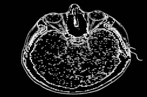 |
Fig. (4). Quadtree decomposed image with 1x1 and 2x2 blocks preserved. |
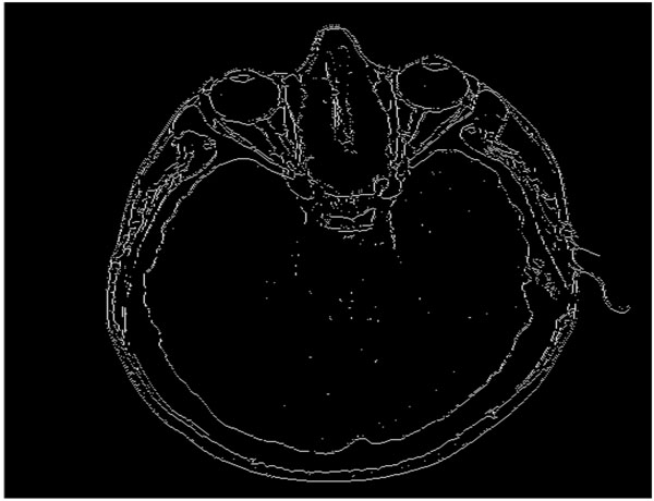 |
Fig. (5). Block diagram demonstrating the various phases of the proposed algorithm. |
The block diagram (see Fig. 6) provides an overview of the phases of the proposed algorithm. With the aid of quadtree decomposition, we eliminate those areas or pixels in an image along which there is little or no variation among intensities. As discussed in Section 1, quadtree decomposition is a recursive hierarchical decomposition of an image into four equal regions, and the division process is performed until all the pixels within a block satisfy a homogeneity condition [8]. The homogeneity condition used in this algorithm implies that no two pixels within a block should have an intensity difference greater than a predefined threshold value τ (also referred to as threshold in the remaining part of the paper). This condition helps us to identify the pixels that qualify as edges, because the 1x1 blocks obtained after the decomposition indicate that the adjacent 1x1 blocks differ in intensity greater than a threshold value. This scenario occurs at an edge.
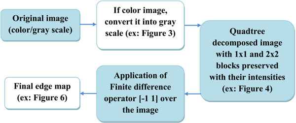 |
Fig. (6). Final edge map of the image given in Fig. (3). |
4. FORMAL DEFINITION OF THE ALGORITHM
The quadtree decomposition forms the first phase of the algorithm. After the decomposition is performed, we obtain the information from the various blocks, including the intensities of the pixels within those blocks. Because the required difference between the intensities is not found within those blocks that contain dimensions of 4x4 or higher, those differences are formulated as zeroes. Finally, we obtain a quadtree-decomposed image with only 1x1 blocks and 2x2 blocks as demonstrated in Fig. (5). By taking both 1x1 and 2x2 blocks, we avoid many of the false dismissals that are observed by only taking 1x1 blocks and we obtain thinner edges than if we process only 2x2 blocks.
|
Algorithm: Quad_Edge_Detection
Input: Mandatory: The grayscale image ‘I’ (or color image, but color image gets converted into grayscale) whose dimensions are mxn where m and n are power of 2, in which edges are to be detected. Optional: The threshold value ‘τ’ used for homogeneity condition (HC) for quadtree decomposition. (Default τ=0.1) Output: The edge map ‘EM’ for the given ‘I’, i.e., image containing the edges of ‘I’. Procedure: Step 1: Ensure ‘I’ is gray scale image: Given ‘I’ checked if it is gray-scale. If not then it is convert into a image. Step 2: Ensuring dimensions are to the power of 2: Given ‘I’ and its dimensions mxn. If m and n not powers of 2, then pad with zeroes Step 3: Perform Quadtree decomposition of ‘I’ The image ‘I’ is decomposed using quadtree decomposition at threshold ‘τ’. The resultant is a spare matrix ‘S’. For every node of ‘S’ (of dimension sz x sz). If sz >2, then all the pixels within the block is made 0. Step 4: Perform pixel scan with specified threshold ‘τ’. For each block of sz <= 2 Perform pixel to pixel scan on the quadtree decomposed image Perform [-1 1] gradient operation on pixels adjacent to non-zero pixels in both x and y direction. If HC {difference between the intensities of pixels}>τ then In x direction: If HC of pixelabove>pixel then mark as an edge pixel. Set the two horizontal neighboring pixels of the edge pixel=0 In y direction: If HC of pixelright> pixel then mark as an edge pixel. Set the two vertical neighboring pixels of the edge pixel=0 |
For the third step of the algorithm, we need to identify the actual pixels from the edge. For this step, we employ a finite difference operator [-1 1] to scan along the x and y directions successively. In our approach, the original image is not replaced, but the edge map is replaced with the final values. Traversing the quadtree-decomposed image that contains only the 1x1 and 2x2 block pixels along with their intensities and for every obtained consecutive non-zero pixel completes this exchange. We apply the [-1 1] operator, and if the difference between the intensities is greater than a value (threshold -7). False dismissals are reduced using the principle that edges are perpendicular to the gradient. As a result, the pixel above the one with greater intensity is marked as an edge pixel and its horizontal adjacent pixels are marked as zero. The same process is repeated in the ‘y’ direction, and the vertical adjacent pixels of the marked edge pixel are made zeroes in the edge map. The final edge map is obtained as demonstrated in the block diagram in Fig. (5).
Unlike Canny [9], this algorithm does not involve the preprocessing for smoothing and does not involve hysteresis. Therefore, only one parameter is required in this case, whereas, three parameters are required in the Canny approach.
5. RESULTS
The method described in the previous sections has been tested on clinical images from various sources. Quadtree decomposition was applied to these images, and a sample set of outputs is shown below (see Figs. 7-11). As seen, each image was processed at varied thresholds. The algorithm was implemented using MATLAB on a 2 GHz Pentium 4 processor with 512 MB RAM.
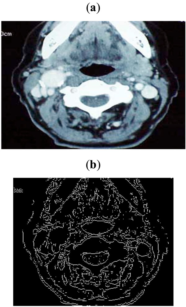 |
Fig. (7). (a) Sample image taken from Peripheral Vascular Surgical and Society, (b) Edge map obtained with threshold of 0.1. |
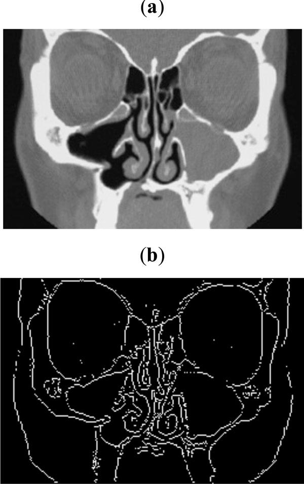 |
Fig. (8). (a) Sample CT scan for sinus, (b) Edge map obtained with threshold of 0.09. |
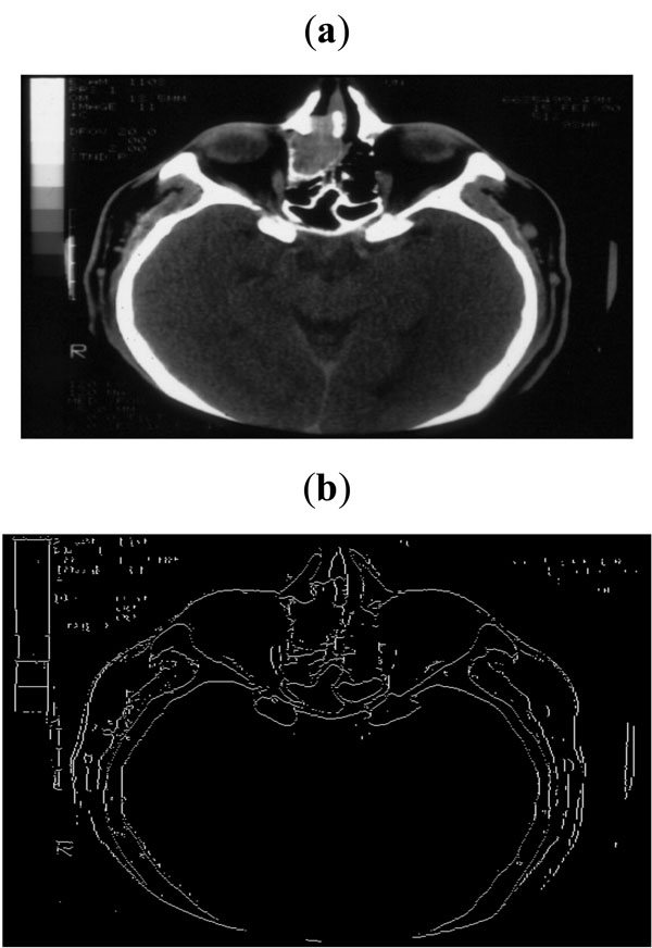 |
Fig. (9). (a) Sample CT scan of head, (b) Edge map obtained with threshold of 0.07. |
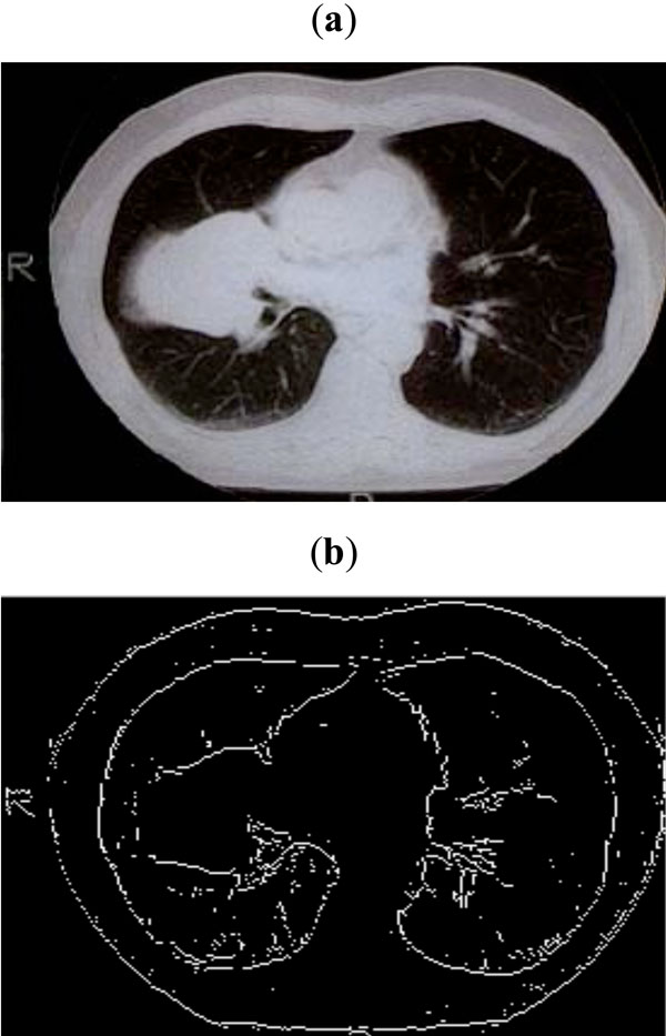 |
Fig. (10). (a) CT scan of lungs, (b) Edge map obtained with threshold of 0.09. |
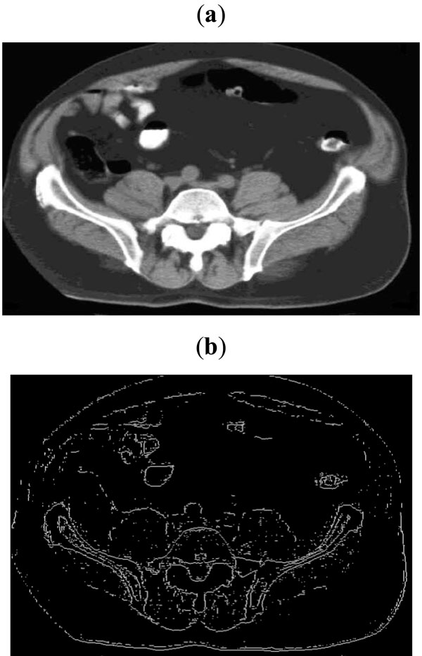 |
Fig. (11). (a) Sample CT scan image, (b) Edge map obtained with threshold of 0.06. |
Theoretically, the complexity of the algorithm is O (nlogn) where ‘n’ is the size of the image after padding zeroes. However, the actual execution time of our algorithm is faster than the Canny execution time in MATLAB, because our algorithm skips the smoothing and hysteresis phases, thus saving the time involved in examining three scans of the image. The following table shows the execution times taken by the Canny approach and by our approach.
5.1. Performance Measures
To further gauge the performance of the algorithm, we tested it using images of two publically available databases, DRIVE and STARE. The DRIVE database contains 40 color images of the retina, with 565x584 pixels and 8 bits per color channel, represented in LZW compressed TIFF format.
These images were originally captured using a Canon CR5 nonmydriatic 3 charge-coupled device (CCD) camera at 45° field of view, and were initially saved in JPEG-format. Besides the color images, the database includes masks with the delimitation of a field of view (FOV) of approximately 540 pixels in diameter for each image, and binary images with the results of manual segmentation. These binary images have already been used as ground truth for performance evaluation of several vessel segmentation methods [17]. The 40 images were divided into a training set and a test set by the authors of the database. The results of the manual segmentation are available for all images in both sets. For the images of the test set, a second independent manual segmentation also exists. To evaluate the performance of our approach, we use all the images of the test set [18].
The other 20-image set, originally collected by Hoover et al., [19] was obtained from the STARE database [20]. These retinal images were captured using a TopCon TRV-50 fundus camera at 35° FOV, and afterwards were digitized to 700x605 pixels, 8 bits per RGB channel. Binary images with manual segmentations are available for each image of the set. We derived the mask images from the matched spatial filter (MSF) images accessible at the STARE project website, with an approximate 650x550 diameter FOV.
The method for the automatic segmentation of the retinal vasculature was evaluated on the images of DRIVE and STARE databases. To facilitate the comparison with other retinal vessel segmentation algorithms, we have selected the segmentation accuracy as a performance measure. The accuracy is estimated by the ratio of the total number of correctly classified points (sum of true positives and true negatives) to the number of points in the image FOV. Other important measures are sensitivity and specificity, which are indicators of the number of properly classified pixels in the true positive and true negative classes. Sensitivity is also known as the true positive fraction, while specificity is known as the true negative fraction, which stands for the fraction of pixels erroneously classified as vessel points. The gold standard for computing the performance measures is a manual segmentation result provided together with each database image.
Table 1 presents the maximum average accuracy and standard deviation calculated with our method for the test set of the DRIVE database, along with the values for the fraction of pixels erroneously classified as vessel pixels, known as the false positive fraction (FPF) and for the percentage of pixels correctly classified as vessel pixels, known as the true positive fraction (TPF). We provide comparison with other methods using the DRIVE database in Table 1.
The results obtained for the 20-image set of the STARE database are shown in Table 2. As in the DRIVE database, the same set of parameters was used for calculating the mean values of the performance measures of average accuracy, true positive fraction (TPF), and false positive fraction (FPF).
Performance of Vessel Segmentation Methods (DRIVE Images)
| Method | Average Accuracy (Standard Deviation) | True Positive Fraction | False Positive Fraction |
|---|---|---|---|
| 2nd Human Observer [18] | 0.9473 (0.0048) | 0.7761 | 0.0275 |
| Mendonca (Grey Intensity) [21] | 0.9463 (0.0065) | 0.7315 | 0.0219 |
| Mendonca (Green Channel) [21] | 0.9452 (0.0062) | 0.7344 | 0.0236 |
| Staal [22] | 0.9442 (0.0065) | 0.7194 | 0.0227 |
| Niemeijer [18] | 0.9417 (0.0065) | 0.6898 | 0.0304 |
| Proposed Method | 0.9840 (0.0266) | 0.7279 | 0.1233 |
Performance of Vessel Segmentation Methods (STARE Images with FOV)
| Method | Average Accuracy (Standard Deviation) | True Positive Fraction | False Positive Fraction |
|---|---|---|---|
| 2nd Human Observer [18] | 0.9354 (0.0171) | 0.8949 | 0.061 |
| Mendonca (a* Component) [21] | 0.9479 (0.0123) | 0.7123 | 0.0242 |
| Mendonca (Luminance) [21] | 0.9421 (0.0151) | 0.6764 | 0.0266 |
| Mendonca (Green) [21] | 0.9440 (0.0142) | 0.6996 | 0.027 |
| Hoover [19, 20] | 0.9267 (0.0099) | 0.6751 | 0.0433 |
| Staal [22] | 0.9516 (not available) | 0.697 | 0.019 |
| Proposed Method | 0.989325 (0.0030) | 0.892065 | 0.048395 |
A comparison of execution time of the proposed quad_edge_detection algorithm with the more traditional Canny algorithm, on different scans (Figs. 7-11) is shown in Fig. (12). The results of edge detection on diabetic retinal images are shown in Fig. (13). The algorithm was executed on an independent set of images under a fixed threshold of τ = 0.06.
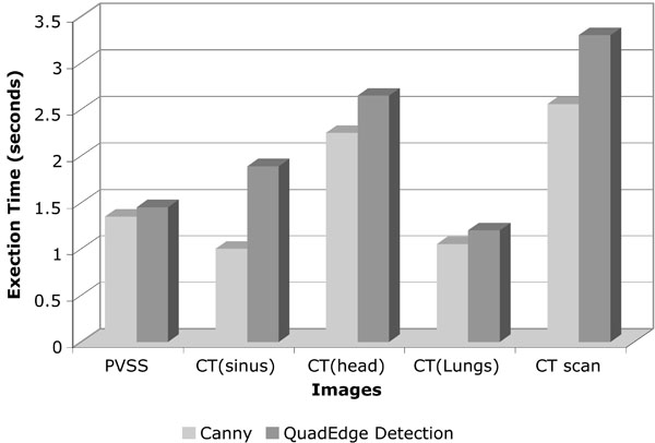 |
Fig. (12). Graph comparing the execution time taken by Canny approach with the proposed algorithm. |
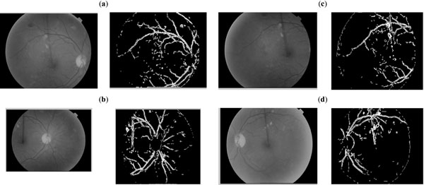 |
Fig. (13). Performance evaluation of the proposed quad_edge_detection algorithm on four independent Retinal scan images. |
6. CONCLUSIONS
We have presented a novel algorithm for edge detection, significant for exploratory analysis and data mining applications in medical image domains. The algorithm employs hierarchical decomposition using quadtrees and post-filtration of edges using finite difference operators. The algorithm efficiently decreases false dismissals of predominately significant edges and significantly lowers the false alarms found in classical approaches. The algorithm is faster than the existing approaches and has reduced storage requirements for the edge map. Our aims for future investigation in this arena include automatically pre-determining the threshold of the quad_edge_detection algorithm and tuning the algorithm for hyper-spectral images originating in clinical domains and confocal images with skewed edge boundaries.
ACKNOWLEDGEMENTS
This research project was supported by the National Science Foundation (NSF) Award No. EPS-0701491 and National Institutes of Health (NIH) Award No. P20 RR16456. Its contents are solely the responsibility of the authors and do not necessarily represent the official views of the National Science Foundation or the National Institutes of Health.
REFERENCES
| [1] | Paulinas M, Usinskas A. A survey of genetic algorithms applications for image enhancement and segmentation Information Technol Control 2007; 36: 278-84. |
| [2] | Senthilkumaran N, Rajesh R. A study on edge detection methods for image segmentation I In: Proceedings of the International Conference on Mathematics and Computer Science (ICMCS-2009); 2009; pp. : 255-9. |
| [3] | Pellegrino FA, Vanzella W, Torre V. Edge Detection Revisited IEEE Trans Syst Man Cybernetics Part B Cybernetics 2004; 34(3): 1500-8. |
| [4] | Senthilkumaran N, Rajesh R. Edge detection techniques for image segmentation - a survey In: Proceedings of the International Conference on Managing Next Generation Software Applications (MNGSA-08); 2008; pp. 749-60. |
| [5] | Rhee I, Martin GR, Muthukrishnan S, Packwood RA. Quadtree-structured variable-size block-matching motion estimation with minimal error IEEE Trans Circuits Syst Video Technol 2000; 1: 42-9. |
| [6] | Bohm C, Berchtold S, Keim DA. Searching in high-dimensional spacers: Index structures for improving the performance of multimedia databases ACM Comput Surv (CSUR) 2001; 33(3): 322-73. |
| [7] | Samet H. Spatial Data Structures, Reading. Addison-Wesley/ACM 1995. |
| [8] | Chen S-K. An exact closed-form formula for d-Dimensional quadtree decomposition of arbitary hyperrectangles IEEE Trans Knowl Data Eng 2006; 18(6): 784-98. |
| [9] | Canny JF. A computational approach to edge detection IEEE Trans Pattern Anal Mach Intell 1986; 8: 679-98. |
| [10] | Rosin Pl, Ioannidis E. Evaluation of global image thresholding for change detection Pattern Recognit Lett 2003; 24: 2345-56. |
| [11] | Prewitt JMS. Object enhancement and extraction In: Lipkin BS, Ed. Picture Processing and Psychopictorics. New York: Academic Press 1970; pp. 75-149. |
| [12] | Kirbas C, Quek F. A Review of Vessel Extraction technique and algorithms ACM Comput Surv (CSUR) 2004; 36(2): 81-121. |
| [13] | Withey DJ, Koles ZJ. Medical images segmentation: methods and software 1 In: I Proceedings of NFSI & ICFBI; 2007; pp. : 140-3. |
| [14] | Iyengar SS, Ed. Structuring of complex bio-systems Chapman and Hall/CRC Press 1991; II. |
| [15] | Senthilkumaran N, Rajesh R. A study on edge detection methods for image segmentation I In: Proceedings of the International Conference on Mathematics and Computer Science (ICMCS-2009); 2009; pp. : 255-9. |
| [16] | Smith SM, Brady JM. SUSAN--a new approach to low level image processing Int J Comput Vis 1997; 23: 45-78. |
| [17] | Niemeijier M, Staal J, van Ginneken B, Loog M, Abramoff MD. Comparitive study of retinal vessel segmentation methods on a new publicly available database In: Fitzpatrick M, Sonka M, Eds. 5370 In: Proceedings SPIE Medical Imaging; 2004; pp. : 648-56. |
| [18] | Niemeijier M, van Ginneken B. DRIVE database 2002 [Online]. Available from: http://www.isi.uu.nl/Research/Databases/DRIVE/ results.php [Accessed: 28 September 2009]; |
| [19] | Hoover A, Kouznetsova V, Goldbaum M. Locating blood vessels in retinal images by piecewise threshold probing of a matched filter response IEEE Trans Biomed Eng 2000; 19: 203-11. |
| [20] | Hoover A. STARE database [Online]. Available from: http://www.parl.clemson.edu/stare/probing/ [Accessed: 28 September 2009]; |
| [21] | Mendonca AM, Campilho A. Segmentation of retinal blood vessels by combining the detection of centerlines and morphological reconstruction IEEE Trans Med Imaging 2006; 25(9): 1200-3. |
| [22] | Staal J, Abramoff MD, Niemeijer M, Viergever MA, Van Ginneken B. Ridge-based vessel segmentation in color images of the retina IEEE Trans Med Imaging 2004; 23(4): 501-9. |


