
RESEARCH ARTICLE
Segmentation of Fluorescence Microscopy Cell Images Using Unsupervised Mining
Xian Du1, Sumeet Dua*, 1, 2
Article Information
Identifiers and Pagination:
Year: 2010Volume: 4
First Page: 41
Last Page: 49
Publisher Id: TOMINFOJ-4-41
DOI: 10.2174/1874431101004020041
Article History:
Received Date: 10/10/2009Revision Received Date: 15/11/2009
Acceptance Date: 15/11/2009
Electronic publication date: 28/5/2010
Collection year: 2010
open-access license: This is an open access article licensed under the terms of the Creative Commons Attribution Non-Commercial License (http://creativecommons.org/licenses/by-nc/3.0/) which permits unrestricted, non-commercial use, distribution and reproduction in any medium, provided the work is properly cited.
Abstract
The accurate measurement of cell and nuclei contours are critical for the sensitive and specific detection of changes in normal cells in several medical informatics disciplines. Within microscopy, this task is facilitated using fluorescence cell stains, and segmentation is often the first step in such approaches. Due to the complex nature of cell issues and problems inherent to microscopy, unsupervised mining approaches of clustering can be incorporated in the segmentation of cells. In this study, we have developed and evaluated the performance of multiple unsupervised data mining techniques in cell image segmentation. We adapt four distinctive, yet complementary, methods for unsupervised learning, including those based on k-means clustering, EM, Otsu’s threshold, and GMAC. Validation measures are defined, and the performance of the techniques is evaluated both quantitatively and qualitatively using synthetic and recently published real data. Experimental results demonstrate that k-means, Otsu’s threshold, and GMAC perform similarly, and have more precise segmentation results than EM. We report that EM has higher recall values and lower precision results from under-segmentation due to its Gaussian model assumption. We also demonstrate that these methods need spatial information to segment complex real cell images with a high degree of efficacy, as expected in many medical informatics applications.
1. INTRODUCTION
Microscopic imaging is nearly ubiquitous in several medical informatics disciplines, including but not limited to, cancer informatics, neuro-informatics, and clinical decision support in ophthalmology. While fluorescence microscopes permit the collection of large, high-dimensional cell image datasets, their manual processing is inefficient, irreproducible, time-consuming, and error-prone, prompting the design and development of automated, efficient, and robust processing to allow analysis for high-throughput applications. The sensitive and specific detection of pathological changes in cells requires the accurate measurement of geometric parameters. Previous research has shown that geometric features, such as shape and area, indicate cell morphological changes during apoptosis [1]. As a precursor to geometric analysis, segmentation is often required in the first processing step. Cell image segmentation is challenging due to the complex morphological cells, illuminant reflection, and inherent microscopy noises. The characteristic problems include poor contrast between cell gray levels and background, a high number of occluding cells in a single view, and excess homogeneity in cell images due to irregular staining among cells and tissues.
Typically, image segmentation algorithms are based on local image information, including edge or gradient, level set [2], histogram [3], clusters [4], and prior knowledge [5]. These segmentation methods have been broadly implemented in medical imaging applications [6]. The current segmentation algorithms used in cell images include seeded watershed [7], Voronoi-based algorithm [8], histogram-based clustering [9] or threshold [10] and active contour [11]. Watershed algorithms can split the connected cells but can lead to over-segmentation. Histogram-based image segmentation is unparametric and based on unsupervised clustering. The histogram is used to approximate the probability density distribution of the image intensity. Pixels in one image are partitioned into several non-overlapping intensity regions. K-means and EM are extensions of histogram segmentation. In EM [9], the distribution of image intensity is modeled as a random variable, which is approximated by a mixture Gaussian model. Due to the lack of intensity distribution information in an image, the EM model can lead to significant bias. of the EM model is computationally efficient and easy to implement, but performs poorly in finding the optimal threshold between clusters in the histogram. Otsu’s optimal threshold is obtained by minimizing intra-class variance and has been applied in nucleus segmentation [12]. Level set and active contour are applied with arbitrary interaction energy in order to split the connected cells in [11]. This method is not meaningful for isolated cells and makes the cell segmentation dependent on cell sizes. In [8], cells are segmented according to the defined metric, the Voronoi distance between pixels and seeds. This metric includes the information from image edges and inter-pixel distance within the image. The parametric active contour and repulsive force are incorporated in [13]. However, this metric is not suitable for the segmentation of a large number of cells in one image.
Unsupervised learning can be adapted and developed for nuclei and cell image segmentation due to the inherent coherent detection and decomposition challenges in the detection and separation of segments. However, it is difficult to select a robust and reproducible method due to the lack of the comparative evaluation of those algorithms. This problem arises partially due to the lack of benchmark data or because of manually outlined ground truth. This paucity of performance evaluation elevates the difficulty for medical scientists to select a suitable segmentation method in medical image applications. Sometimes, methods are selected based on intuition and experience; e.g., Otsu’s threshold is used broadly in nuclei image segmentation. Moreover, no broadly acceptable method can address the nuclei and cell image segmentation problems in a diverse range of applications accurately and robustly. Recently, several synthetic (e.g. [14]) and benchmark cellular image data (e.g. [15]) have been made publicly available.
In this paper, we present and evaluate the performance of several unsupervised data mining techniques in cell image segmentation. We adapt four distinctive, yet complementary, methods for unsupervised learning, including those based on k-means clustering, EM, Otsu’s threshold, and GMAC. Validation measures are defined to compare and contrast the performance of these methods using publicly available data. It should be noted that the segmentation algorithms are typical representatives of methods based on histogram, model, threshold, and active contour. We only focus on segmentation methods using low-level image information, such as pixel intensity and image gradient. GMAC represents both the snake and level set technologies [14]. The results presented in this paper can guide domain users to select suitable segmentation methods in medical imaging applications.
2. UNSUPERVISED MINING METHODS FOR IMAGE SEGMENTATION
Let us consider an image I of size r = M × N pixels, where each pixel can take L possible grayscale-level values in the range [0, L - 1]. Let h(x) be the normalized histogram of the image I.
2.1. Notation
| xi | Intensity value of pixel i |
| h(x) | Histogram of the image I,x ∈ [0,L-1] |
| r | Image size in terms of pixel numbers |
| Tr (I) | Transformation function of image I |
| pj (xi; θj) | j-th probability density function with parameter set θj |
| μj | Mean of cluster j |
| ∑j | Variance of cluster j |
 |
Within-class variance, Between-class variance. |
| ω (T)i=1,2 | Probabilities of the two clusters separated by threshold T |
| f (x) | Image expressed with spatial term x, which refers to pixel location |
| λ (in GMAC) | Scalar that controls the balance between regularization and data |
2.2. K-Means Clustering
We use K-means clustering for image segmentation to find the optimal threshold, such that the image feature values of pixels on one side of the threshold are closer to their feature values’ mean than the distance between those feature values and the means on the other side of the threshold. This method is performed using the histogram of image intensity. We assume that the image intensities compose a vector space and try to find natural clustering in it. The pixels are clustered around centroid ci, which are obtained by minimizing the objective function
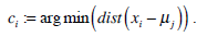 |
(1) |
The centroid for each cluster is iteratively obtained as follows,
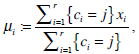 |
(2) |
where r is the image size in terms of pixel number, i iterates over all intensities, j iterates over all centroids, and μi are the centroid intensities. Using intensity value directly in microscopic cell image segmentation will not lead to the desired segmentation result due to the dynamic ranges, which vary in images. We propose a gray-level transformation function in the form Tr(I) = I r for the above algorithm to implement k-means segmentation in cell image I, where γ is a positive constancy.
2.3. Expectation Maximization Method
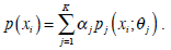
The Expectation Maximization (EM) algorithm assumes that an image consists of a number of gray-level regions, which can be described by parametric data models. When the histogram of the gray levels is regarded as an estimate of the probability density function, the parameters of the function can be estimated for each gray-level region using the histogram. The objective of the EM algorithm is to find the maximum likelihood estimates of the parameters in the function. Correspondingly, EM consists of two steps: expectation and maximization. Using the same notations in Section 2.1, the mixture of probability density functions is as follows,
 |
(3) |
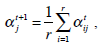
In the above, α j is the proportion of the j-th density function in the mixture model, and  is the j-th density function with parameter set θj. The Gaussian mixture model (GMM) is the most employed in practice, and has two parameters, mean µ j and covariance ∑j, such that θ j = (µj, ∑ j) . We consider GMM in our research. If we assume that θ tj is the estimated value of parameters θ j = (µj, ∑ j), obtained at the t-th step, then
  can be obtained iteratively. The EM algorithm framework follows,
 |
(4) |
 |
(5) |
 |
(6) |
 |
(7) |
These equations state that the estimated parameters of the density function are updated according to the weighted average of the pixel values where the weights are obtained from the E step for this partition. The EM cycle starts at an initial setting of
 and updates the parameters using Equations ((4)-(7)) iteratively. The EM algorithm converges until its estimated parameters cannot change. Then, the final parameters,
 are applied in image segmentation by labeling pixels using Maximum Likelihood (ML). Pixel xi is labeled using the following function,
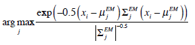 |
(8) |
2.4. Threshold-Based Segmentation
Threshold segmentation is a method that separates an image into a number of meaningful regions through the selected threshold values. If the image is a grey image, thresholds are integers in the range of [0, L-1], where L-1 is the maximum intensity value. Normally, this method is used to segment an image into two regions: background and object, with one threshold. The following is the equation for threshold segmentation:
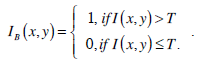 |
(9) |
In the above equation, IB is the segmentation resultant. The most famous threshold method was proposed by Otsu in [12]. The Otsu’s method finds the optimal threshold T among all the intensity values from 0 to L-1 and chooses the value that produces the minimum within-class variance
 as the optimal threshold value. Consequently, the optimal value of TOpt is obtained through the following optimal computation,
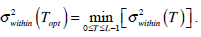 |
(10) |
In the whole image, variances σ2 are made up of two parts:
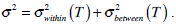 .
Otsu shows that
.
Otsu shows that  is the same as
  . Therefore, the optimal value of T can also be obtained through the following alternative optimization process:
 |
(11) |
Equation (11) is often used to find the optimal threshold value for simple calculation. Theoretically,  is expressed in the following,
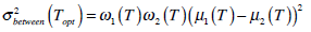 |
(12) |
where  are the probabilities of the two clusters separated by threshold T, and μi(T)i=1,2 are the cluster means. ωi(T)i=1,2 and μi(T)i=1,2
can be estimated using histogram h(x) as follows,
are the probabilities of the two clusters separated by threshold T, and μi(T)i=1,2 are the cluster means. ωi(T)i=1,2 and μi(T)i=1,2
can be estimated using histogram h(x) as follows,
 |
(13) |
 |
(14) |
 |
(15) |
 |
(16) |
Using the above Equations (12)-(16), the optimal threshold T is exhaustively searched among [0, L-1] to meet the objective according to Equation (11).
2.5. Global Minimization of the Active Contour Model (GMAC)
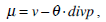
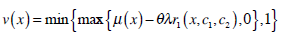
We choose the global minimization of the active contour model (GMAC) [16] to analyze the implementation of active contour in cell-image segmentation. This method has a simple initialization and fast computation, and it can avoid being stuck at an undesired local minima. GMAC is based on Mumford and Shah’s (MS) function and the Chan and Vese’s model of active contours without edges (ACWE) [17]. GMAC improves ACWE by using weighted total variation and dual formulation of the TV form, which preserves the advantage of ACWE. We define GMAC and related concepts below.
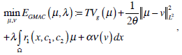 |
(17) |
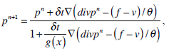
where r1 (x, c1, c2) = ((c1-f(x))2 - (c2-f (x)2))dx, f(x) is the given image, and c1 and c2 are constants calculated for partitioning in iteration; e.g., if , µ* = arg minE2 [µ,v,c1,c2], c1 and c2 are the means of pixels in two partitions and can be obtained using equations, θ > 0 is chosen small enough, λ > 0 is a parameter controlling scale related to the scale of observation of solution, and α is constant.
 |
(18) |
where g(x) is an edge indication function which gives a link between snake model and region terms. The minimization Equation (17) is solved using the following equations iteratively until convergence:
 |
(19) |
 |
(20) |
 |
(21) |
 |
(22) |
 |
(23) |
In Equation (21), δ t is the time step.
3. EXPERIMENTAL RESULTS
In this section, we present the experimental results from the segmentation of three types of fluorescent cellular images: synthetic cell images, nuclei images with ground truth, and brain cell microscopic images. The first two types of image data are used to evaluate the quantitative performance of the four segmentation methods and to compare the results to the ground truth. The brain cell images are segmented with qualitative performance analysis due to the lack of ground truth.
3.1. Quantitative Measure
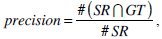
We use the traditional precision, recall, and F-score as the quantitative measures in pixel level. These measures are standard techniques used to evaluate the quality of the segmentation results against the ground truth. These measures quantify discrepancy between segmentation results and binary ground truth mask as follows:
 |
(24) |
 |
(25) |
 |
(26) |
where SR is the segmentation result and GT is the ground truth of images. The symbol ‘#’ refers to the pixel numbers in the sets.
3.1.1. Segmentation of Synthetic Data
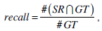
Benchmark sets of synthetic cell population images with ground truth are simulated by P. Ruusuvuori in [18]. We select the second benchmark set which consists of multi-channel cell images because we do not have suitable real cell images with ground truth for evaluation. In this set, nuclei, cytoplasm, and subcellular components have been simulated by tuning parameters such as size, location, randomness of shape, and other background or fluorescence parameters (see details in [18]). The image sets are divided into two subsets: high quality and low quality (examples shown in Fig. 1), each consisting of 20 cell images. The second set has overlapping cells and a noisy background. Each image contains 50 cells. As each simulated image has a corresponding binary mask as ground truth, binary operations can easily calculate the quantitative measure defined above.
 |
Fig. (1). Synthetic cell images a) (low quality) with noisy background and overlapping cells, b) (high quality) without noise in background and overlapping cells, c) ground truth of image a, d) ground truth of image b. |
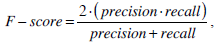
Fig. (2) shows the segmentation result of four methods for the low quality synthetic image data in Fig. (1a). Segmented images in Fig. (2) are compared and evaluated using the ground truth image in Fig. (1c). Fig. (3) shows the segmentation result of four methods for the high quality synthetic image data in Fig. (1b). Segmented images in Fig. (3) are compared and evaluated using the ground truth image in Fig. (1d).
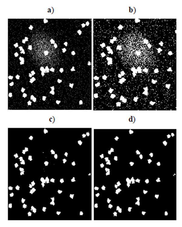 |
Fig. (2). Segmentation result for synthetic cell images of low quality in Fig. (1a). a) K-means result, b) EM result, c) Otsu’s result, d) GMAC result. |
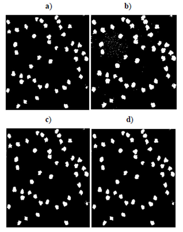 |
Fig. (3). Segmentation result for synthetic cell image of high quality in Fig. (1b). a) K-means result, b) EM result, c) Otsu’s result, d) GMAC result. |
Figs. (4-6) and Table 1 are the quality measure values for the segmentation results using subcellular images with low quality. Figs. (7-9) and Table 2 are the quality measure values for the segmentation results using subcellular images with high quality.
Average Measures of the Segmentation Methods Applied on High Quality Synthetic Cell Images
| F-Score | Precision | Recall | |
|---|---|---|---|
| K-Means | 0.9745 | 0.9726 | 0.9765 |
| EM | 0.9040 | 0.8267 | 0.9986 |
| Otsu’s | 0.9738 | 0.9798 | 0.9679 |
| GMAC | 0.9703 | 0.9874 | 0.9538 |
Average Measures of the Segmentation Methods Applied on Low Quality Synthetic Cell Images
| F-Score | Precision | Recall | |
|---|---|---|---|
| K-Means | 0.9350 | 0.9530 | 0.9180 |
| EM | 0.5331 | 0.3821 | 0.9915 |
| Otsu’s | 0.9269 | 0.9295 | 0.9259 |
| GMAC | 0.9445 | 0.9781 | 0.9133 |
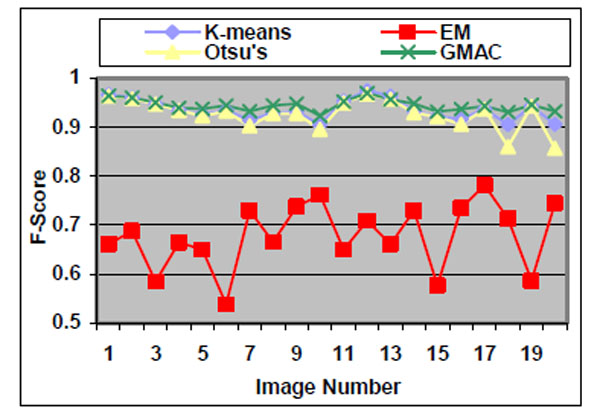 |
Fig. (4). F-score of the four methods applied on low quality simulated cell images. |
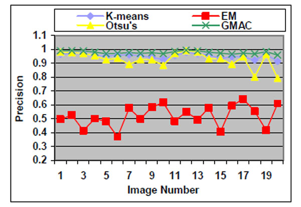 |
Fig. (5). Precision of the four methods applied on low quality simulated cell images. |
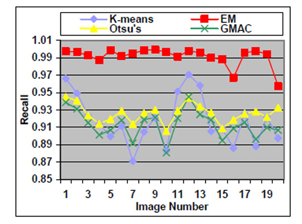 |
Fig. (6). Recall of the four methods applied on low quality simulated cell images. |
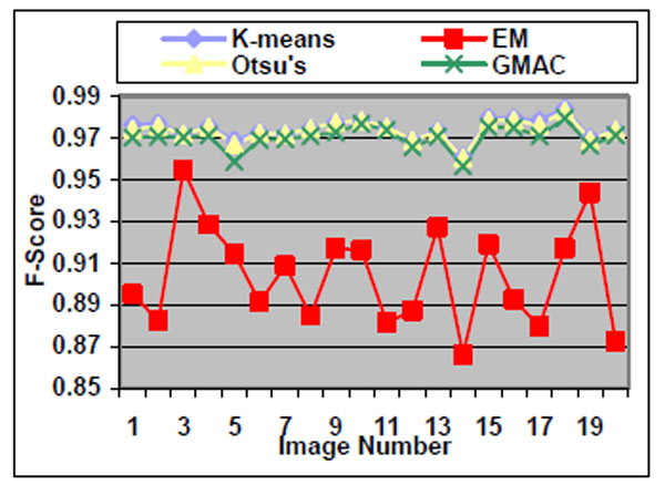 |
Fig. (7). F-score of the four methods applied on high quality simulated cell images. |
 |
Fig. (8). Precision of the four methods applied on high quality simulated cell images. |
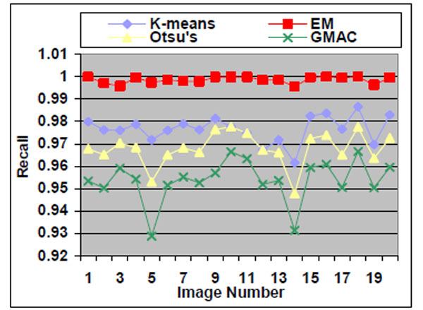 |
Fig. (9). Recall of the four methods applied on high quality simulated cell images. |
We observe that the segmentation results of lower quality images, with noisier backgrounds and overlapping cells, have worse results than those in high quality images. K-means, Otsu’s threshold and GMAC obtain similar segmentation quality in both sets of images, measured by F-score, precision, and recall. Their performance is more robust against noises than EM. Moreover, the EM algorithm has lower precision, while keeping much higher recall values, especially for cell images with noisy backgrounds. To further understand these phenomena, real nucleus images are segmented in the next section.
3.1.2. Segmentation of Nucleus Images
Sixteen nucleus images were hand-outlined by an expert in the CellProfiler project [8, 15]. We use these images to evaluate the segmentation algorithms quantitatively. We obtain similar results, as shown in Figs. (10-13), as those we obtained in Section 3.1.1. We observe in Table 3 that EM maintains higher recall and lower precision values, even if its F-score values are as high as the other segmentation methods in several images. From Fig. (10d), we can see that the EM under-segments nucleus images strongly, which induces the high recall values. This under-segmentation is due to the presumed dual Gaussian mixture models in the calculation of EM. One model represents background, and the other refers to objects. When objects have much smaller grayness regions than background (as shown in Fig. 10a), the dual Gaussian mixture model leads to under-segmentation.
Average Quality Measures of the Segmentation Methods on Nucleus Images
| F-Score | Precision | Recall | |
|---|---|---|---|
| K-Means | 0.8714 | 0.8766 | 0.8668 |
| EM | 0.7473 | 0.6131 | 0.9664 |
| Otsu’s | 0.7976 | 0.9475 | 0.6910 |
| GMAC | 0.7880 | 0.8880 | 0.7148 |
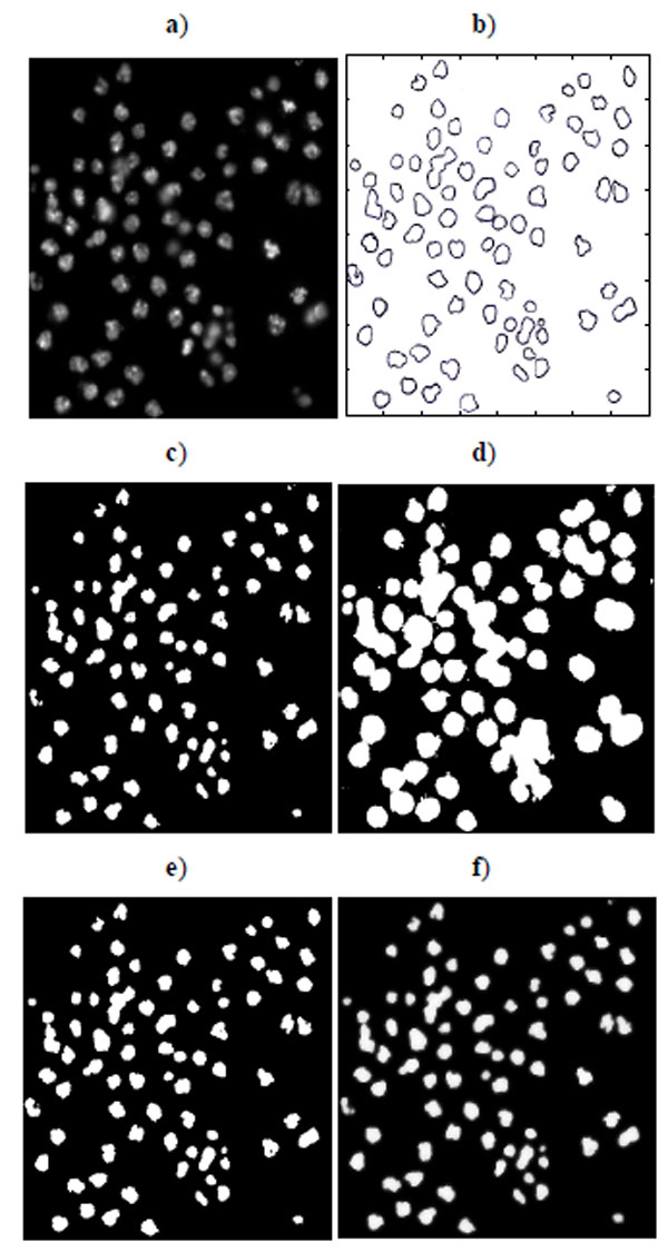 |
Fig. (10). Segmentation of nucleus images: a) Nucleus images, b) Ground truth, c) K-means result, d) EM result, e) Otsu’s result, and f) GMAC result. |
 |
Fig. (11). F-score of the four methods applied on nucleus images. |
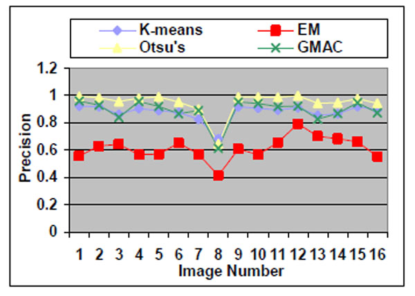 |
Fig. (12). Precision of the four methods applied on nucleus images. |
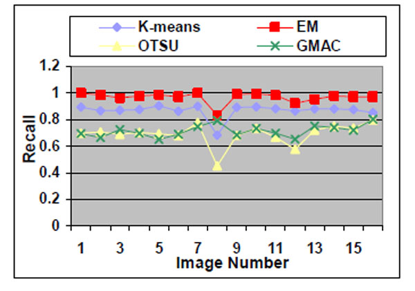 |
Fig. (13). Recall of the four methods applied on nucleus images. |
Otsu’s method also has drawbacks. Although it performs well for nucleus segmentations, due to its fastness and simplicity in application, it cannot be proven the best segmentation method for nucleus images. As shown in Section 3.1.1, Otsu’s method shows stable precision and recall values even when it encounters arbitrarily defined noises. However, in the experiment using real nucleus images, the Otsu’s method recall value is significantly lower than its precision values, which means it has over-segmented the image.
GMAC is more robust and stable than the Otsu’s method in our experiments. GMAC depends on both image intensity distribution information (region) and gradient (edge) information. When the contrast between background and cells becomes light, and cells are hidden by noises, the combination of gradient and intensity information records better information than intensity alone does, e.g. in Otsu’s. In the k-means method, we choose k=2 to cluster some objects into one group and other segments into a background group. K-means performs the best in almost all experiments. Its good performance is due to the application of power function for the compensation of intensity transformation brought in by the microscopic device. In this research, we assume this power function is known, and we obtain it by choosing the optimal k-means result (smallest error between k-means segmentation result and ground truth). It demonstrates that the k-means method can obtain robust and precise segmentation results with the aid of power function.
3.2. Quality Measure of Segmentation of Brian Cell Images
In this evaluative study, brain cell images were captured using a computer controlled Microscope (Leica DMI 6000 Digital). The cell images are of a normal healthy astrocytes cell, which has been stained with Calcein AM, a vital dye that stains only living cells. The test images are 1040 ↔ 1392 pixels with 8-bit gray-levels. As no manual outlining has been performed on the images, the performance of segmentation methods is qualitatively evaluated.
As shown in Fig. (14a), brain cell images are dark, and cell contours are blurred. The segmentation results of k-means, Otsu’s, and GMAC (Fig. 14b, 14d, 14e) seem to be washed out. Using the nucleus, light areas, we can identify the existing cells in the image. The segmentation result of GMM EM (Fig. 14c) is still under-segmented. In Fig. (15), we can see that the background, denoted by the annotated line marked by ‘*’, has a narrow estimated intensity distribution while cells distribute in a wider intensity levels, denoted by the other annotated line marked by ‘+’. This presentation using standard Gaussian distribution leads to errors in the estimate of probability distribution. As shown in Fig. (16), the individual intensity distributions are summed to obtain the mixed Gaussian distribution, which is presented by the annotated line marked by square. The errors in estimation are accumulated in the sum procedure, which can be presented by the discrepancy between the areas covered by the estimated distribution and the true intensity distribution denoted by the annotated line marked by triangle. The other three segmentation results have cells split with the nucleus, although several cells are over-segmented. This over-segmentation can be explained as that these techniques consider image intensity and texture information in the segmentation process, while the spatial relation or some connection between pixels is missed. Moreover, compared to the synthetic images in Section 3.1.1, real cell images are more complex and difficult to segment.
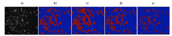 |
Fig. (14). a) Brain cell microscopy image, b) K-means clustering result, c) EM clustering result, d) Otsu’s segmentation result, e) GMAC segmentation result. |
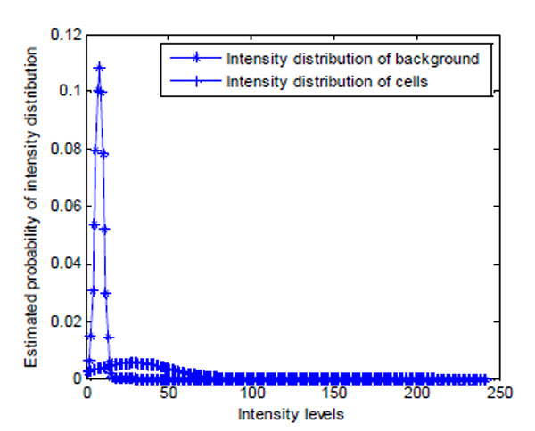 |
Fig. (15). Estimated intensity distribution of image in Fig. (14a) using GMM EM model. |
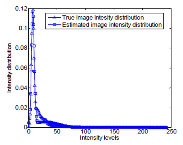 |
Fig. (16). The ground truth and estimation of the intensity distribution of image in Fig. (14a). |
4. CONCLUSION
We present four unsupervised mining methods in cell image segmentation. The four methods are compared and contrasted to showcase efficacy strengths, as well as embedded limitations. While no single method outperforms the others in all tests, this analysis is expected to assist image scientists in improving these techniques for the more complex cell image segmentation problems encountered in related disciplines.
The methods are evaluated both quantitatively and qualitatively using synthetic simulated and real images. EM performs weakly in both cases due to its presumed Gaussian model. It needs a better model assumption in microscopic imaging if applied in cell image segmentation. Otsu’s method cannot always guarantee a good segmentation result, especially when the contrast between the background and cells is poor. GMAC integrates intensity and gradient information and keeps a stable performance in our experiments. K-means can perform robust segmentation with the aid of power function. In future work, spatial information between pixels must be involved to improve the performance of those techniques. The knowledge about the cell images, such as inclusion of the power distribution function will be incorporated in segmentation.
REFERENCES
| [1] | Jean RP, Gray DS, Spector AA, Chen CS. Characterization of the nuclear deformation caused by changes in endothelial cell shape J Biomed Eng 2004; 126(5): 552-8. |
| [2] | Osher S, Sethian JA. Fronts propagating with curvature-dependent speed: Algorithms based on Hamilton-Jacobi formulations J Comput Phys 1988; 79: 12-49. |
| [3] | Ohlander R, Price K, Reddy DR. Picture segmentation using a recursive region splitting method Comput Graph Image Process 1978; 8: 313-3. |
| [4] | Jain AK. Data Clustering: 50 Years Beyond K-Means. Technical Report TR-CSE-09-11 Pattern Recognit Lett 2009. sin press |
| [5] | Cootes T, Taylor CJ, Cooper DH, Graham J. Active shape models-Their training and application CVGIP: Image Understanding 1995; 61: 38-59. |
| [6] | Pham ZL, Xu C, Prince JL. Current methods in medical image segmentation Ann Rev Biomed Eng 2000; 2: 315-7. |
| [7] | Wahlby C, Lindblad J, Vondrus M, Bengtsson E, Bjorkesten L. Algorithms for cytoplasm segmentation of fluorescence labelled cells Anal Cell Pathol 2002; 24(2-3): 101-1. |
| [8] | Jones TR, Carpenter A, Golland P. Voronoi-based segmentation of cells on image manifolds Lect Notes Comput Sci 2005; 535-43. |
| [9] | Bazi Y, Rruzzone L, Melgani F. Image thresholding based on the EM algorithm and the generalized Gaussian distribution Pattern Recognit Lett 2007; 40: 619-34. |
| [10] | Otsu N. A threshold selection method from Gray-level Histogram IEEE Trans Syst Man Cybernetics 1979; 1: SMC-9. |
| [11] | Yan PK, Zhoum XB, Shahm M, Wongm STC. Automatic segmentation of high-throughput rnai flurescent cellular images IEEE Trans Inf Technol Biomed 2008; 12(1): 109-7. |
| [12] | Coulot L, Kischner H, Chebira A, et al. Topology preserving STACS segmentation of protein subcellular location images In: Proc IEEE Int Symp Biomed Imging ; Apr 2006; Arlington, VA. 566-9. |
| [13] | Zimmer C, Labruyere E, Meas-Yedid V, Guillen N, Olivo Marin J-C. Segmentation and tracking of migrating cells in Videomirco-scopy with parametric active controus: a tool for cell-based drug testing IEEE Trans Image Process 2002; 12(10): 1212-21. |
| [14] | Benchmark set of synthetic images for validationg cell image analysis algorithms: Benchmark images Available from: http://www.cs.tut.fi/sgn/csb/simcep/benchmark/ [Accessed: 10 September 2009]; |
| [15] | Cell Profiler: Cell image analysis software Available from: http://www.cellprofiler.org/ [10 September 2009]; |
| [16] | Bresson X, Esedoglu S, Vandergheynst P, Thiran J, Osher S. Fast Global Minimization of the Active Contour/Snake Model J Math Imaging Vis 2007; 28(2): 151-67. |
| [17] | Chan TF, Vese LA. Active contours without edges IEEE Trans Image Process 2001; 10(2): 266-77. |
| [18] | Ruusuvuori P, Lehmussola A, Selinummi J, Rajala T, Huttunen H, Yli-Harja O. Benchmark set of synthetic images for validating cell image analysis algorithms In: Proceedings of the 16th European Signal Processing Conference (EUSIPCO-2008); Lausanne, Switzerland. 2008. |