
RESEARCH ARTICLE
Meta-Analysis of Multi-Arm Trials Using Empirical Logistic Transform
Hathaikan Chootrakool, Jian Qing Shi*
Article Information
Identifiers and Pagination:
Year: 2008Volume: 2
First Page: 112
Last Page: 116
Publisher Id: TOMINFOJ-2-112
DOI: 10.2174/1874431100802010112
Article History:
Received Date: 27/3/2008Revision Received Date: 05/5/2008
Acceptance Date: 19/5/2009
Electronic publication date: 6/6/2008
Collection year: 2008
open-access license: This is an open access article licensed under the terms of the Creative Commons Attribution Non-Commercial License (http://creativecommons.org/licenses/by-nc/3.0/) which permits unrestricted, non-commercial use, distribution and reproduction in any medium, provided the work is properly cited.
Abstract
Meta-analysis of multi-arm trials has been used increasingly in recent years. The aim of meta-analysis for multi-arm trials is to combine evidence from all possible similar studies. In this paper we propose normal approximation models by using empirical logistic transform to compare different treatments in multi-arm trials, allowing studies of both direct and indirect comparisons. Additionally, a hierarchical structure is introduced in the models to address the problem of heterogeneity among different studies. The proposed models are performed using the data from 31 randomized clinical trials (RCTs) which determine the efficacy of antiplatelet therapy in maintaining vascular patency.
1. INTRODUCTION
Most meta-analysis has focused on summarising of treatment effect measures based on comparisons of two treatments. Some meta-analysis data sets contain information on more than two treatments comparing evidence of multi-arm trials comparisons. This type of data is called Multi-arm trials in this paper although some authors call it mixed treatment comparison (MTC). Higgins and Whitehead [1] presented a random effect meta-analysis for binary data and introduced an idea of ‘borrowing strength’ from indirect comparison. They considered using the general parameter approach and the exact binomial approach to estimate parameters of interest in a meta-analysis. Lu and Ades [2] proposed a Bayesian hierarchical model using the Markov Chain Monte Carlo to represent meta-analysis of multi-arm trials. Inconsistency in multi-arm trials evidence structure was examined by Lu and Ades [3]. They performed a Bayesian hierarchical model with fixed effects or random effects for fitting multi-arm trials under the assumption that the available evidence sources were consistent in estimating all treatment contrasts.
In meta-analysis for comparing two treatments, we usually collected all the studies providing information on comparing those two treatments directly. However some studies in multi-arm trials give a useful information on indirect comparison in a situation where the treatments have not been directly compared. Thus, there are two types of treatment comparisons in meta-analysis of multi-arm trials: one is to compare two treatments directly, the other is to use information from indirect comparisons. For example, from antiplatelet data given in Table 2, there are three groups of studies available: treatments A, B and C; the control group of the meta-analysis is treatment C, studies in group GAB compare treatment A versus B, studies in group GBC compare treatment B versus C, and studies in group GCA compare treatment C versus A and our aim is to compare treatment A versus B. The studies in group GBC and GCA then provide the indirect comparison for treatment A versus B. Later in this paper, we will blur the concept between direct and indirect comparisons since our model can actually give estimate of the treatment effect between any two arms of all treatments involved in the multi-arm trials.
Results for the empirical log-odds ratio models
| Model | δAB | δAC | δBC | |||
|---|---|---|---|---|---|---|
| µAB | τAB | µAC | τAC | µBC | τBC | |
| Model 1 | 0.108146 | 0.275320 | -0.568930 | 0.275320 | -0.677076 | 0.275320 |
| (SD) | (0.156391) | (0.136747) | (0.161554) | (0.136747) | (0.150660) | (0.136747) |
| OR scale | 1.114210 | 1.316952 | 0.566130 | 1.316952 | 0.508100 | 1.316952 |
| Model 2 | 0.064521 | 0.09338 | -0.599244 | 0.333440 | -0.663766 | 0.318274 |
| (SD) | (0.053287) | (0.065361) | (0.171172) | (0.228035) | (0.187616) | (0.204939) |
| OR scale | 1.066648 | 1.097879 | 0.549226 | 1.395761 | 0.5149085 | 1.37475 |
| Model 3 | 0.062605 | 0.00000009 | -0.590714 | 0.335648 | -0.653320 | 0.212374 |
| (SD) | (0.252691) | (0.324800) | (0.262792) | (0.502075) | (0.241205) | (0.218013) |
| OR scale | 1.064607 | 1.0 | 0.553931 | 1.398847 | 0.520315 | 1.23661 |
The direct and indirect comparisons for RCTs in a meta-analysis have been expressed by several authors [2-6]. In this paper we propose a normal approximation model based on the empirical logistic transform. There are at least two advantages comparing to other methods: (1) the proposed empirical log-odds ratio models exclude the trial effects and then it will give an unbiased estimate for treatment effect while the other methods may give a biased estimates in some circumstances (see for example the discussion on page 59 in [7]); (2) The computation is very efficient and fast. The method has been used for the systematic reviews of antiplatelet trialists’ collaboration [8] which investigates the efficacy of antiplatelet therapy in maintaining vascular patency in various categories of patients. The paper is organized as follows. We begin by introducing the data structure of multi-arm trials and performing empirical log-odds and empirical log-odds ratio models in Section 2.1. The maximum likelihood method is illustrated in Section 2.2. The last section concludes the ideas of this paper and gives some comments.
2. METHODOLOGY
In this section we shall propose our ideas of empirical log-odds and empirical log-odds ratio models through the antiplatelet data. Clinically, after coronary artery revascularisation of patients, whether by coronary artery bypass grafting or by percutaneous transluminal coronary angioplasty, angiographic studies show substantial rates of re-occlusion [9]. Experimental and clinical evidence suggests that antiplatelet therapy may help prevent vascular graft or arterial occlusions, particularly during the period soon after vascular procedures, before any intimal damage has healed [10, 11]. The data was analyzed in order to determine the efficacy of antiplatelet therapy in maintaining vascular patency. There are 31 RCTs in total investigating the use of aspirin plus dipyridamole, or aspirin alone, in the comparison with the control group. The trials compare three treatments A (aspirin plus dipyridamole), B (aspirin only) and C (control group), where 6 trials (1-6) compare A, B and C, 4 trials (7-10) compare A and B, 13 trials (11-24) compare A and C and 7 trials (25-31) compare B and C. The data is shown in Table 2.
Randomized Trials of Aspirin Data
| Study Number | Aspirin + Dipyridamole (A) event/total | Aspirin (B) event/total | Control (C) event/total |
|---|---|---|---|
| 1 | 15/49 | 10/47 | 18/51 |
| 2 | 35/162 | 37/155 | 47/153 |
| 3 | 83/368 | 85/373 | 114/371 |
| 4 | 23/100 | 16/100 | 39/100 |
| 5 | 6/16 | 2/16 | 12/17 |
| 6 | 0/100 | 6/100 | 12/100 |
| 7 | 20/60 | 22/64 | |
| 8 | 26/313 | 27/317 | |
| 9 | 10/41 | 6/40 | |
| 10 | 8/55 | 15/55 | |
| 11 | 33/160 | 37/160 | |
| 12 | 37/202 | 81/205 | |
| 13 | 4/18 | 9/30 | |
| 14 | 17/62 | 20/63 | |
| 15 | 8/61 | 24/64 | |
| 16 | 13/47 | 27/46 | |
| 17 | 21/34 | 14/35 | |
| 18 | 11/72 | 15/68 | |
| 19 | 6/187 | 13/189 | |
| 20 | 86/286 | 86/263 | |
| 21 | 4/33 | 15/32 | |
| 22 | 15/50 | 12/50 | |
| 23 | 7/22 | 19/31 | |
| 24 | 15/132 | 13/67 | |
| 25 | 15/71 | 16/71 | |
| 26 | 6/29 | 15/31 | |
| 27 | 7/68 | 17/69 | |
| 28 | 24/215 | 47/213 | |
| 29 | 19/148 | 28/150 | |
| 30 | 6/19 | 18/25 | |
| 31 | 2/47 | 11/45 |
2.1. Models
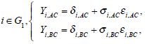
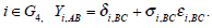
For convenience, we partition the data set into four groups. Let G1 = {1, ...,6}, G2 = {7, ...,10 }, G3 = {11, ...,24} and G4 = {25,...,31} be four sets of studies comparing treatment A versus B versus C, A versus B, A versus C and B versus C, respectively. Let riA, riB and riC be the numbers of patients that have reocclusions on treatments A, B and C respectively where the ith study is in
G1 ⋃ G2 ⋃ G3, G1 ⋃ G2 ⋃ G4 and G1 ⋃ G3 ⋃ G4, respectively, where
Grespectively, where ‘⋃’ stands for ‘and’. The total numbers of patients are niA, niB and niC, respectively. Let πiA, πiB and πiC be the probabilities of patients that have reocclusions on treatments A, B and C respectively in the ith study. The riA, riB and riC are thus binomially distributed as Bin(πiA, niA), Bin(πiB, niB) and Bin(πiC, niC) respectively. Suppose that XiA, XiB and XiC are the empirical logistic transforms, called the empirical log-odds for (riA, niA), (riB, niB) and (riC, niC) respectively, where for example the empirical logistic transform of XiA is defined by log(riA + 0.5)/(niA − riA + 0.5) (we may also use notation ln (·) here) where i is in the set
G1 ⋃ G2 ⋃ G3. From Cox and Snell [7, page 31], if riA is not too small or not too close to niA, the empirical logistic transform XiA has an approximation normal distribution with mean log(πiA/(1 − πiA)). The variance can be estimated from the data:
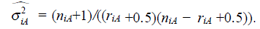 It iA is the same for XiB and XiC. The models on the log-odds scale for each group are defined as follows
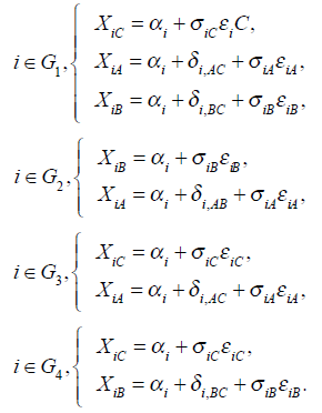
The above models are called empirical log-odds models. The σ2iA,, σ2iB, and σ2iC, are the variances of empirical log-odds XiA, XiB and XiC, respectively. The εiA, εiB and εiC are independent and follow the standard normal distribution and correspond to the random sampling errors of the models XiA, XiB and XiC within the ith study respectively. All random sampling errors are therefore independent and normally distributed as N(0, σ2iA,), N(0, σ2iB,) and N(0, σ2iC,) respectively. The δi,AC, δi,BC and δi,AB are the treatment effects, which are defined, for example
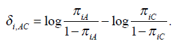
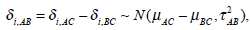
It is called log-odds ratio between treatment A and treatment C, measuring the effect of treatment A comparing to the control group C. This is the parameter of interest. The main purpose of the meta-analysis is to find the overall estimates of the log-odds ratios between treatments A versus C, B versus C and A versus B. We may assume a fixed effect or a random effect. The fixed effect model assumes that all the δi,AC’s are the same as δAC, where δAC is a fixed treatment effect between the treatment A and the control group C for all studies in G1 and G3.The fixed treatment effect δBC can be considered in the same way. It is important to note that the treatment effect δi,AB or its fixed effect δAB is not a free parameter since δAB = δAC − δBC.
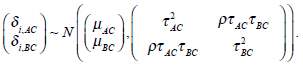
To address the problem of between-study heterogeneity, we usually use a random effect model, i.e. assume δi,AC, δi,BC and δi,AB are random variables. If we use a normal distribution, the random effect model is to assume that the treatment effects δi,AC, δi,BC and δi,AB are normally distributed as 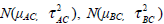 and
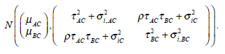
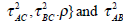
and 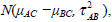 respectively. For the studies involved in G1, the treatment effects δi,AC and δi,BC are defined based on the same baseline treatment C and therefore may be dependent. Let ρ be the correlation coefficient between the treatment effects δi,AC and δi,BC, we may define a model as
 |
(1) |
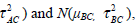
The parameters μAC and μBC are the overall mean effects between the control group C and the treatment A, and the control group C and the treatment B, respectively. The τ2AC and τ2BC measure the between-study heterogeneity of the treatment effects δi,AC and δi,BC, respectively. The correlation coefficient ρ measures the amount of linear association between δi,AC and δi,BC.In group G2, treatments A and B are involved. From (1), we have
 |
(2) |
where 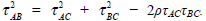 The entries on the diagonal of the covariance matrix in (1) are often called the heterogeneity parameters of the treatment effects in a meta-analysis. The useful property of the model parame terisation is the correlation structure of the covariance matrix. An important special case is that the heterogeneity parameters of the treatment effects are assumed to be the same, i.e. τAC = τBC = τAB, called homogeneity of variances. Hence the correlation coefficient ρ takes the value 1/2 because the treatment effects δi,AC and δi,BC involve the control group C in the same way. A general model is to allow the heterogeneity parameters of the treatment effects to be different for each treatment effect related to the control group, called heterogeneity of variances.The covariance matrix will be in the standard form as shown in (1) and (2).
The αi in each group is the trial effect. We can consider the following two assumptions. The first one is that the trial effects are assumed to be study-level effects, which means the αi’s are different fixed parameters. We need to include 31 different unknown parameters in the model. The second one is that we may assume a model for αi’s. A special case is to assume that all trial effects are the same: α = α1 = α2 = . . . = α31. Conversely if the trial effect is assumed to be a random effect, we may assume that 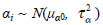 where μα is the overall mean of the trial effects and τα measures the magnitude of the variation between the studies. The standard random effect model used in meta-analysis was described by [12]. To capture skewness and heavy tails in the distribution of the trial effect, we may use a mixture of normal distributions [13]. However, in practice the trial effects in most meta-analysis would not satisfy any model since different experiment designs and different data analysis models are used in different studies. Most of the existed methods therefore used the first assumption. Note that the number of unknown parameters is the same as the number of studies. This will result in some theoretical and computational problems. The accuracy of the estimation depends on the sample size of each study not the overall sample size of the pool in the meta-analysis. The estimates of some parameters may not be consistent. Due to the large number of parameters, the computation is usually unstable. We therefore propose the following empirical log-odds ratio model. Based on the empirical log-odds models, a model on the log-odds ratio scale is suggested here. Let Yi, AC = XiA − XiC, Yi, BC = XiB − XiC and Yi, AB = XiA − XiB, which are called as the empirical log-odds ratio for XiA versus XiC, XiB versus XiC, and XiA versus XiB, respectively. The models on the log-odds ratio scale in each group can be defined as follows
 |
(3) |
 |
(4) |
 |
(5) |
 |
(6) |
The above models are called empirical log-odds ratio models. The trial effect αi’s are no longer in the above models. Note that the models Yi,AC and Yi,BC for the studies in G1 are not independent. The treatment effects δi,AC and δi,BC are jointly normally distributed as shown in (1). The σ2AC, σ2BC and σ2AB are variances of the log-odds ratios Yi,AC, Yi,BC and Yi,AB respectively, which can be calculated from σ2AC, σ2BC and σ2AB by for example σ2i,AC = σ2iA + σ2iC. Consequently the empirical log-odds ratio model (Yi,AC, Yi,BC)t for studies in G1 is distributed as
 |
(7) |
The μAC and μBC are the overall mean effects for the models Yi,AC and Yi,BC. The variances of the models Yi,AC and Yi,BC are τ2AC + σ2i,AC and τ2BC + σ2i,BC respectively. The covariance between both models is 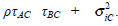 . Additionally the empirical log-odds ratio models for G2, G3 and G4 are normally distributed as
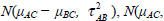
 , respectively.
2.2. Estimation
To make inference, the maximum likelihood method is applied to estimate the unknown parameters in the empirical log-odds ratio models given in (3)-(6). Our aim is to estimate the unknown parameters for the meta-analysis consisting of 31 studies. Let θ be the collection of all unknown parameters for the meta-analysis. Suppose that θ can take any value within admissible ranges Θ. The method of maximum likelihood is to find the value  within Θ which makes the likelihood function of θ as large as possible. The log-likelihood function for the empirical log-odds models can be written as
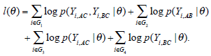
Notice that the l(θ) is a summation of log-likelihoods from G1 to G4.The p(Yi,AC, Yi,BC|θi), p(Yi,AB|θi), p(Yi,AC|θi) and p(Yi,BC|θi) represent the joint probabilities or likelihoods of observing the data that has been collected in G1, G2, G3 and G4 respectively. Maximizing the log-likelihood function, we use the function nlme in the software R to solve the unknown parameters. As described in the previous section, there are two assumptions of heterogeneity parameters: homogeneity and heterogeneity variances. For the model with homogeneity variances (Model 1 in Table 1), we assume that τAC = τBC = τAB and the correlation coefficient between the treatment effects takes 1/2. For the model with heterogeneity variances (Model 2 in Table 1), the correlation coefficient is an unknown parameters. Thus, the θ in Model 1 is {μAC, μBC, τ2} while θ in Model 2 is 
 is given in (2).
2.3. Numerical Results
The estimates of unknown parameters in Model 1 and Model 2 are shown in (Table 1). From Model 1, the overall means of treatment effects A versus B, A versus C and B versus C are 0.108146, -0.568930 and -0.677076 respectively and the variation between studies in those comparisons are assumed the same, 0.275320. The overall means estimated from Model 2 are quite similar. Those means for Model 2 are 0.064521, -0.599244 and -0.663766, and the variation between studies are 0.09338, 0.33440 and 0.318274 respectively. The correlation coefficient in Model 2 is 0.96. Notice that the estimator of ρ is quite close to one and τAB is very small. All treatment effects are on the log-odds ratio scale. In term of interpretation, we consider the overall means on the odds ratio (OR) scale. The results obtained from both models are quite close. They indicate that both treatment A and treatment B reduce the rates of reocclusion significantly by about 40% comparing to control group. However, the difference between treatment A and treatment B is neglect although treatment B is even slightly better than treatment A (improve by about 14% using Model 1 and 6% using Model 2). In both models, we used empirical log-odds ratio models to eliminate the nuisance parameters (trial effects). The computation is very efficient and very stable, it converges very fast for almost any starting points.
3. CONCLUSION
We demonstrated a normal approximation model based on empirical logistic transform to multi-arm trials data. The approximation is usually quite good if the number of observations in each study is not too small (the number of samples in a single study should usually be larger than 20). Since the normal distribution is used, the calculation from the normal approximation is much faster than from the model with exact binomial distributions. It takes just about 2 seconds using Model 1 for the example discussed in this paper, but it takes about 30 minutes if we use the exact binomial distributions and conditional likelihood approach (it takes about 5 minutes if an unconditional likelihood approach is used, but this method needs to estimate αs’s). The final results from both models are very close.
The estimation of ρ is quite trick. In our example, the information for ρ or τAB mainly comes from G2.Due to small number of studies involved in G2, we should be careful to explain the values of the estimates, which ρ is quite close to 1 and τ is quite close to zero. In this case, a way is to assume the between-study heterogeneity  of indirect comparison was not relatively estimated from the between-study heterogeneities
  of the direct comparison. This is the Model 3 given in Table 1, which τAB is an independent unknown parameter and ρ is assumed as 1/2. The results from Models 2 and 3 are almost the same. Several authors [4, 6] pointed out in the same way. Whenever there is no or insufficient evidence on direct comparison from RCTs, the indirect comparison may provide useful or supplementary information on the treatment effect. However the validity of the indirect comparisons depends on the internal validity and similarity of the included studies (see [6]). If the trial effects in the empirical log-odds model are assumed to be study-level fixed effects, the estimation is not simple as many parameters are involved in the model. This leaded to a problem of inconsistent estimate. Solving the problem of the trial effect, the empirical log-odds ratio model was suggested in order to eliminate the trial effect from the model. Some other methods can also be used to address the problem, for example, a conditional approach based on the binomial distribution. We will not discuss the details here.
ATC(II) Collaboration [8] concluded that antiplatelet therapy (aspirin plus dipyridamole (A) or aspirin alone (B)) produced a highly significant (2p ≤ 0.00001) reduction in vascular occlusion in a wide range of patients. The odds of vascular graft or arterial occlusion were reduced by about 40% while treatment continued. Our numerical results in the previous section are similar to the conclusion from [8].
ACKNOWLEDGEMENT
HC is supported by a grant from Suan Dusit Rajabhat University (SDU), Thailand.